2. Generating SQW files

This page tells you how to generate a .sqw file from experimental data. There are two different situations when you will want to do this:

Note

You can also generate fake .sqw files from detpar (help dummy_sqw) and some modelling codes can produce .sqw files.

• During an experiment, when you want to accumulate data files into an .sqw file as they are collected - use accumulate_sqw

• When you have a full set of data files already that you want to process in one go - use gen_sqw

The two functions have almost identical syntax, as is explained in the sections below.

To generate the .sqw file, neutron data for each run needs to be provided in one of two formats:

• the legacy ASCII format .spe file, together with an ASCII detector parameter file (the .par file),

• or their replacements the HDF (hierarchical Data Format) .nxspe file. More details about these files and how to create them can be found here.

2.1. accumulate_sqw

This is a way of generating data ‘on the fly’ during an experiment. It saves time by appending new data to an already existing .sqw file.

The syntax is as follows:

accumulate_sqw(spe_file, par_file, sqw_file, efix, emode, alatt, angdeg,...
               u, v, psi, omega, dpsi, gl, gs[, grid_size_in][, urange_in] ...
               [, instrument][, sample][, 'replicate'][, 'clean']);

The input parameters are defined as follows:

• spe_file is a cell array, each element of which is a string specifying the full file name of the input .spe or .nxspe files (e.g. spe_file{1} = 'C:\data\mer12345.spe').

• par_file is a string giving the full file name of the parameter file for the instrument on which the data were taken. This is required for .spe files. For .nxspe files you do not need to specify an instrument parameter file (Provide empty string ‘’ instead), as detector information will be picked up from .nxspe files themselves. If you do specify par_file, the detector info from there will override the information in the .nxspe files.

• sqw_file is a string giving the full file name of the sqw output file you wish to generate.

• efix is the incident neutron energy for each .spe file. If a single incident energy was used for all runs then this number is a scalar, otherwise it must be a vector with the same number of elements are there are .spe files.

• emode is either: - 1 for direct geometry instruments - 2 for indirect geometry.

• alatt is a vector with 3 elements, specifying the lengths in Angstroms of the crystal lattice parameters.

• angdeg is a vector with 3 elements, specifying the crystal lattice angles in degrees.

• u and v are both 3-element vectors. These specify how the crystal’s axes were oriented relative to the spectrometer in the setup for which you define psi to be zero.

  u specifies the lattice vector that is parallel to the incident neutron beam

  v is a second vector in the horizontal plane.

Note

It is not necessary for v to be perpendicular to u.

• psi specifies the angle of the crystal relative to the setup described in the above paragraph (i.e. the angle about the vertical axis through which the sample has been rotated).

Note

If a single orientation of the crystal was used for all measurements then this number can be a scalar, otherwise it is a vector.

Warning

In the case of accumulate_sqw this is a vector listing the expected values of psi that will be used.

It is important to get this about right, as it ensures that the underlying reciprocal space grid in the .sqw file is big enough to encompass all of the data you plan to collect. If it is not, then you lose all the time-saving and the file has to be generated from scratch!

• omega, dpsi, gl, and gs specify the offsets (in degrees of various angles). gl and gs describe the settings of the large and small goniometers. omega is the offset of the axis of the small goniometer with respect to the notional u. Finally dpsi allows you to specify an offset in psi, should you wish. These angle definitions are shown below:

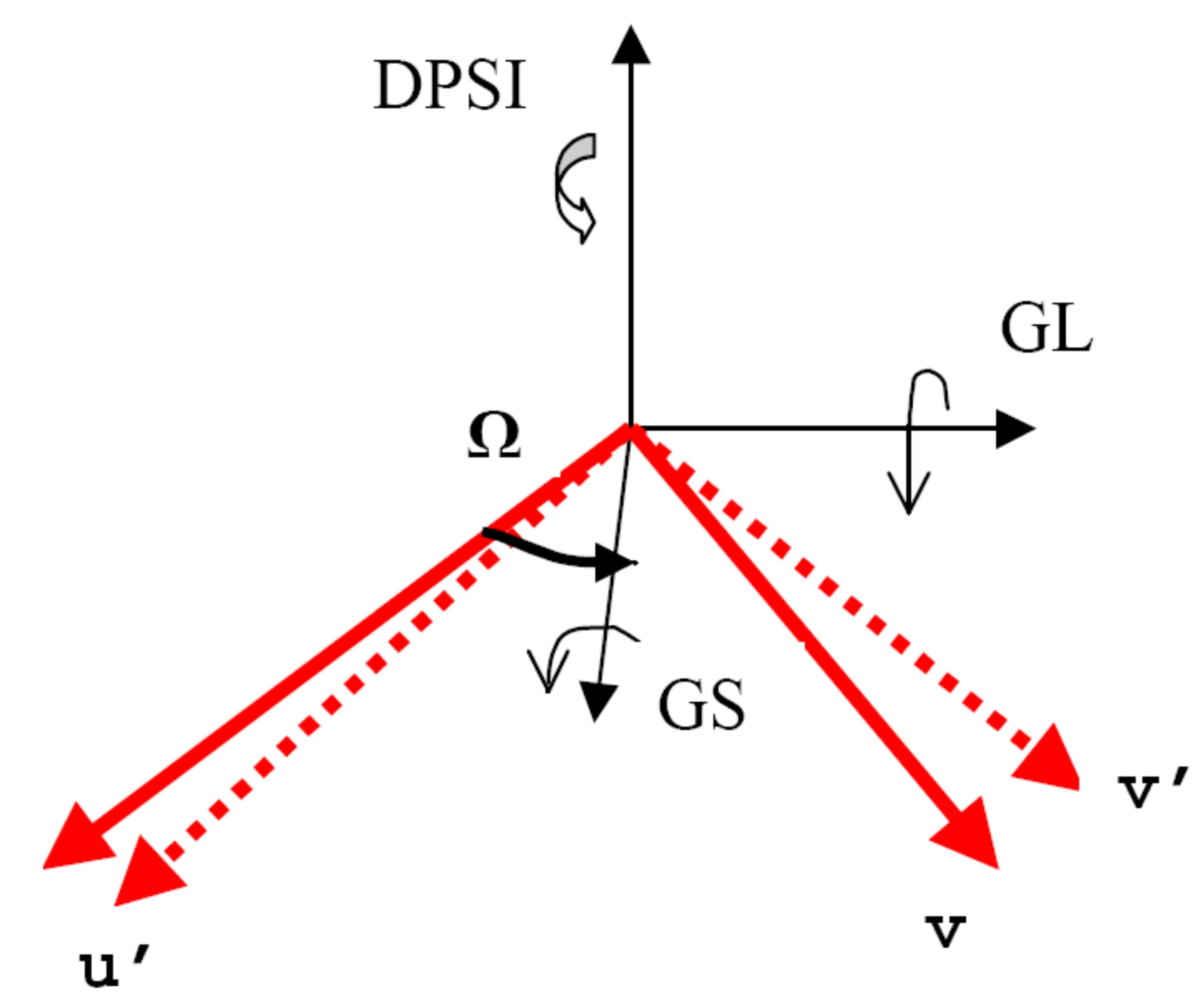
Virtual goniometer angle definitions

The optional input arguments are as follows:

• grid_size_in: A scalar or row vector of grid dimensions. If it is not given, or is left blank (i.e. set to []), the default value will be determined on the number and size of the contributing .spe or .nxspe files.

• urange_in: The range of data grid for output along each Q and E direction as a 2x4 matrix -

  [x1_lo, x2_lo, x3_lo, x4_lo;
   x1_hi, x2_hi, x3_hi, x4_hi]
  

  The default if not given or set to [] is the smallest hypercuboid that encloses the whole data range.

• instrument: A free-format structure or object containing instrument information [scalar or array of length nfile]

• sample: A free-format structure or object containing sample geometry information [scalar or array of length nfile]

• 'replicate': Normally the function forbids an .spe or .nxspe file from appearing more than once. This is to trap common typing errors. However, sometimes you might want to create an .sqw file using, for example, just one .spe file as the source of data for all crystal orientations in order to construct a background from an empty piece of sample environment. In this case, use the keyword 'replicate' to override the uniqueness check.

• 'clean': Create the .sqw file from fresh. This option deletes existing .sqw file (if any) and forces fresh generation of .sqw file from the list of data files provided. It is possible to get confused about what data has been included in an .sqw file if it is built up slowly over an experiment. Use this option to start afresh.

2.2. gen_sqw

This is the main function you will use to turn the data accumulated in multiple .spe files into a single .sqw file that will be used by the rest of the Horace functions. An introduction to its use is given in the getting started section. The syntax is the same as for accumulate_sqw; the only difference is that you give a list of existing input datasets rather than the anticipated list.

The inputs and outputs are of the form:

[tmp_file, grid_size, urange] = gen_sqw (spe_file, par_file, sqw_file, efix, emode, alatt, angdeg, ...
                                         u, v, psi, omega, dpsi, gl, gs ...
                                         [, grid_size_in][, urange_in][, 'replicate']);

Optional input arguments:

• grid_size_in: A scalar or row vector of grid dimensions. If it is not given, or is left blank (i.e. set to []), the default value will be determined on the number and size of the contributing SPE or NXSPE files.

• urange_in: The range of data grid for output along each Q and E direction as a 2x4 matrix - [x1_lo,x2_lo,x3_lo,x4_lo;x1_hi,x2_hi,x3_hi,x4_hi]. The default if not given or set to [] is the smallest hypercuboid that encloses the whole data range.

• instrument: A free-format structure or object containing instrument information [scalar or array length nfile]

• sample: A free-format structure or object containing sample geometry information [scalar or array length nfile]

• 'replicate': Normally the function forbids an SPE or NXSPE file from appearing more than once. This is to trap common typing errors. However, sometimes you might want to create an sqw file using, for example, just one SPE file as the source of data for all crystal orientations in order to construct a background from an empty piece of sample environment. In this case, use the keyword ‘replicate’ to override the uniqueness check.

Optional output arguments:

• tmp_file: A cell array containing the full file names of the temporary files that were created by gen_sqw. These will be deleted if the function ran correctly, but if there was a problem, then they will still exist and it can be useful to know their names so that they can be deleted manually.

• grid_size is a vector with 4 elements which specifies the actual grid size of the output .sqw file that was created. For example, if every data point has the same value of Qz then the third element will be 1.

• urange gives the range in reciprocal space of the data. If urange_in was specified then this will be the same, but if not then it tells you the calculated range of the 4-dimensional hypercuboid which encompasses all of the data.

2.3. Applying symmetry operations to an entire dataset

In the explanation below, we wish to apply symmetrisation to the entire data file. Under the hood, what happens is that the data for each run is symmetrised, and then these symmetrised data are combined to make the sqw file. This avoids the problem of running out of memory when attempting to symmetrise large sections of the unfolded sqw file / object.

To use this functionality, call gen_sqw or accumulate_sqw as above, with the additional argument 'transform_sqw' which takes a function handle:

gen_sqw (spefile, par_file, sym_sqw_file, efix, emode, alatt, angdeg,...
    u, v, psi, omega, dpsi, gl, gs,'transform_sqw',@(x)(symmetrise_sqw(x,v1,v2,v3)))

or more generally

gen_sqw (spefile, par_file, sym_sqw_file, efix, emode, alatt, angdeg,...
    u, v, psi, omega, dpsi, gl, gs,'transform_sqw', @user_symmetrisation_routine)

The first example above would build a sqw file reflected as in the example for the reflection in memory, but with the transformation applied to the entire dataset. In the second, more general, case the user defined function (in a m-file on the Matlab path) can define multiple symmetrisation operations that are applied sequentially to the entire data. An example is as follows, which folds a cubic system so that all six of the symmetrically equivalent (1,0,0) type positions are folded on to each other:

function wout = user_symmetrisation_routine(win)

wout=symmetrise_sqw(win,[1,1,0],[0,0,1],[0,0,0]);   % fold about line (1,1,0) in HK plane
wout=symmetrise_sqw(wout,[-1,1,0],[0,0,1],[0,0,0]); % fold about line (-1,1,0) in HK plane
wout=symmetrise_sqw(wout,[1,0,1],[0,1,0],[0,0,0]);  % fold about line (1,0,1) in HL plane
wout=symmetrise_sqw(wout,[1,0,-1],[0,1,0],[0,0,0]); % fold about line (1,0,-1) in HL plane

see very important notes on the technical details of symmeterising a whole dataset in manual/Symmetrising_etc:Commands for entire datasets.