1. Planning a Horace scan
Note
While Horace includes its own planner it is worth noting that the MANTID DGS planner exists [1].
1.1. horace_planner: a simple scan planner
Horace has a useful little tool which allows you to work out the coverage of reciprocal space that will be achieved for a given instrument, the incident energy and the sample angle range.
You start it up by typing
horace_planner
The graphical user interface shown below should open up
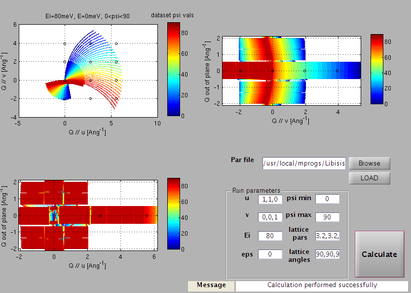
Fig. 1.1 Horace planner GUI
You first select the
.parfile associated with your instrument (which specifies detector positions), by browsing to it, and then clickingLOAD.Next you enter the vector u and v as comma-separated lists.
u is the Q-space direction parallel to the incident beam when the crystal rotation angle, \(\psi\), is equal to 0
v is a second vector not parallel to u lying in the equatorial plane of the detectors (horizontal for most instruments).
Note
It is not necessary for v to be perpendicular to u.
Enter the lattice parameters (in Angstroms) and lattice angles (in degrees) of your sample as comma-separated lists.
Enter the incident energy, \(E_i\), and the energy transfer you are interested in, then the minimum and maximum values of \(\psi\) you are considering.
Now hit
Calculateand the coverage is calculated. The axes of the three plots are the Q directions parallel to u and v, and the out-of-plane direction, respectively. The axes are labelled with inverse Angstroms, and circles are shown at integer \((h,k,l)\) positions.The three views shown in the image above correspond to looking at the Q-coverage volume from three different perspectives.
Top-left we see the view from above (i.e. down an axis perpendicular to u and v)
Top-right we see the view from the right-hand side (i.e. along u from the positive side)
Bottom-left we see a view from the bottom (i.e. along v from the negative side)
1.2. More detailed planning of scans
The scan planner shown above is quick and simple to use, but sometimes you need
greater detail about what reciprocal space coverage you will get for a given
scan. To do this, you can generate a fake dataset, where the signal is
represented as the angle of of the contributing scan at each point.
Note
This process can be rather slow. Often it is better to check using the simple scan planner detailed above first before making decisions.
An example script for generating fake data is given below.
en = [0:10:190];  % energy bins (coarse for simulation)
par_file = '/usr/local/mprogs/Libisis/InstrumentFiles/maps/4to1_124.par';  % detector parameter file
sqw_file_fake = '/home/maps/maps_users/Gruenwald/fake_200meV.sqw';         % name of output file

efix = 200;  % incident energy
emode = 1;   % select 1 for direct geometry spectrometer

alatt = [5.7, 5.7, 5.7];
angdeg = [90, 90, 90];

u = [1, 0, 0];
v = [0, 1, 1];

psi = [-90:0];  % scan range in degrees

omega = 0;
dpsi = 0;
gl = 0;
gs = 0;

dummy_sqw (en, par_file, sqw_file_fake, efix, emode, alatt, angdeg, ...
           u, v, psi, omega, dpsi, gl, gs);
Once you have created this fake dataset you can take cuts and slices out of it in exactly the same way as you would a real dataset. For example:
proj = line_proj([1, 0, 0], [0, 1, 0]);  % viewing axes for plots

my_l = [-2:2];  % loop over a set of values of L

for i = 1:numel(my_l)
    my_slice(i) = cut(sqw_file_fake, proj, [-3, 0.03, 3], [-3, 0.03, 3], [my_l(i)-0.1, my_l(i)+0.1], [80, 90], '-nopix');
    plot(compact(my_slice(i)));
    keep_figure;
end
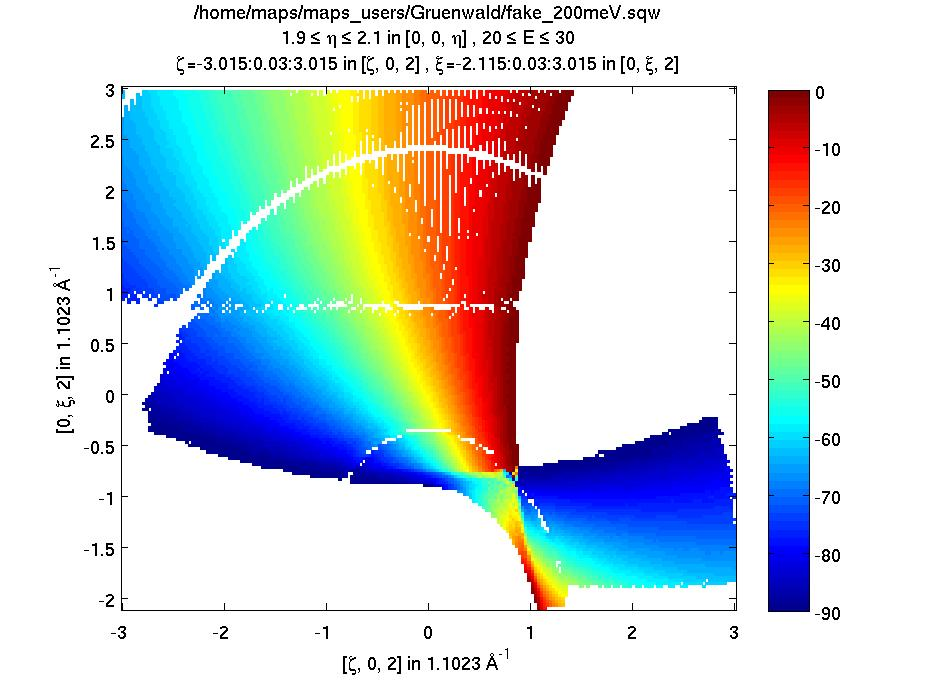
Fig. 1.2 Sample plot of fake dataset