5. Cutting data of interest from SQW files and objects

Horace stores the data produced in a neutron experiment in a 4-D dataset which are called the “pixels”. These represent the neutron events measured during an experiment. The dataset also contains the rest of the full information about the experiment.

Horace also creates a 4-dimensional histogram (binned) of these “pixels” represented in reciprocal space (hkl-dE) which we call the “image”. This carries only limited information about the original data, i.e. only the averaged intensity over the bins remains.

Note

For the differences between dnd and sqw objects see: here

Generally, rather than attempting to deal with the full experimental data, a user works with smaller objects, extracted from the full dataset using cut. This is for multiple reasons including:

• The 4-dimensional dataset is impossible to visualise, as only 3-d (through slice-o-matic), 2-d and 1-d cuts can be easily represented.

• The entire dataset is often too large to fit in the memory of most computers.

5.1. cut

cut takes a (or multiple) section(s) of data from an sqw or dnd object or file, discards the pixels which lie outside of the binning regions (described below) from an sqw and accumulates them into a histogram (the “image” or dnd, which may be independent if requested or attached to the parent sqw). It can return an object or file depending on the parameters given.

cut can produce objects of the same or reduced size and dimensions. The result of a cut is itself an sqw or dnd object which can be further plotted, manipulated, etc.

Note

If the resulting object is estimated by Horace to be too big to fit in memory, it will be saved to disc, but will appear mostly indistinguishable from a memory-backed sqw object, supporting most operations. We call this a “file-backed sqw” (for more detail see: File- and memory-backed cuts). When the manual refers to an sqw object both “file-backed” and “memory-backed” are included.

Warning

File-backed objects may be significantly slower to operate on than memory backed ones.

The inputs are as follows:

my_cut = cut(data_source[, proj], p1_bin, p2_bin, p3_bin, p4_bin[, '-nopix'][, sym][, filename])

where:

• data_source is either a string giving the full filename (including path) of an input sqw file or a variable containing a sqw object.

• proj defines the axes and origin of the cut including the shape of the region to extract and the representation in the resulting histogram.

• pN_bin describe the histogram bins to capture the data.

There are also several extra optional arguments which are:

• -nopix

  drop the “pixels” from the resulting object returning just the dnd binned data (the “image”). This option is faster and the resulting object requires less memory, but is also more restricted in what you can do with the result.

• sym

  cell array of symmetry operations. For a full description of usage, see here.

• filename

  if provided, uses file-backed algorithms to write the resulting object directly to a file named filename and return a file-backed sqw.

Warning

If cut is called without a return argument, the filename option is mandatory.

5.1.1. Data Source

data_source in cut is either a string giving the full filename (including path) of the input .sqw file or just the variable containing an sqw or dnd object stored in memory from which the pixels will be taken.

Warning

By convention both sqw and dnd objects use the .sqw suffix when stored to disc. It is advisable to name the file appropriately to distinguish the types stored inside, e.g. MnO2_sqw.sqw, MnO2_d2d.sqw.

5.1.2. Projection (proj)

The projection defines the coordinate system and thus the meaning of the Binning arguments and the presentation of the data.

proj should be a projection type such as line_proj, sphere_proj, etc. which contains information about the desired coordinate system representation.

Note

To take a cut from an existing sqw or dnd object while retaining the existing projection, provide an empty proj argument:

w1 = cut(w, [], [lo1, hi1], [lo2, hi2], ...)

Different projections are covered in the Projection in more detail section below.

Note

Changing projection does not change the underlying pixels, merely its representation (binning) in the image and how thus it appears when plotted.

It does, however, affect which pixels are selected and which are discarded when making a cut.

5.1.3. Binning arguments

The binning arguments (p1_bin, p2_bin, p3_bin and p4_bin) specify the binning / integration ranges for the Q & Energy axes in the target projection’s coordinate system (c.f. Projection in more detail and changing projections).

Each can independently have one of four different forms below.

Warning

The meaning of the first, second, third, etc. component in pN_bin changes between each form. Ensure that you have the correct value in each component to ensure your cut is what you expect.

• []

  An empty binning range will use the source binning axes in that dimension.

• [step]

  A single (scalar) number defines a plot axis.

  The bin width will be equal to the number you specify. The lower and upper limits will be from the source binning axes in that dimension.

Note

A value of [0] is equivalent to [step] using bin size of the source coordinate system.

Warning

When changing projections e.g. line_proj to sphere_proj, using either [] or [step] see, changing projections below.

• [lower,upper]

  A vector with two components defines an integration axis.

  The signal will be integrated over that axis between the limits specified by the two components of the vector.

Warning

A two-component binning axis defines the integration region between bin edges. For example, [-1 1] will capture pixels from -1 to 1 inclusive.

• [lower,step,upper]

  A vector with three components defines a plot axis.

  The first lower and the last upper components specifying the centres of the first and the last bins of the data to be cut. The middle component specifies the bin width.

Note

If step is 0, the step is taken from the source binning axes.

Warning

A three-component binning axis defines the integration region by bin centres, i.e. the limits of the data to be cut lie between min = lower-step/2 and max = upper+step/2, including min/max values. For example, [-1 1 1] will capture pixels from -1.5 to 1.5 inclusive.

• [lower, separation, upper, cut_width]

  A vector with four components defines multiple integration axes with multiple integration limits in the selected direction.

  These components are:

  • lower

    Position of the lowest cut bin-centre.

  • separation

    Distance between cut bin-centres.

  • upper

    Approximate (see below) position of highest cut bin-centre

  • cut_width

    Width of each cut, centred on each bin-centre, thus extending one half-width in both directions

  The number of cuts produced will be one more than the number of separation-sized steps between lower and upper.

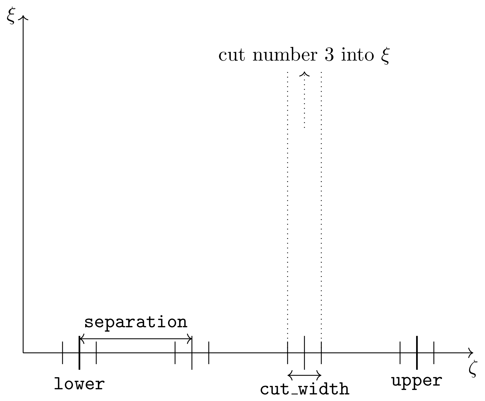
Diagram showing the relationship between the 4 binning parameters and their meaning in the context of a cut, where: lower = 1, upper = 7, separation = 2 and cut_width = 0.6, i.e [1, 2, 7, 0.6]. \(\zeta\) and \(\xi\) are arbitrary axes where \(\zeta\) is the specified axis. This will produce 4 cut objects around 1, 3, 5 and 7.

Warning

upper will be automatically increased such that separation evenly divides upper - lower. For example, [106, 4, 113, 2] defines the integration ranges for three cuts, the first cut integrates the axis over 105-107, the second over 109-111 and the third 113-115.

5.1.4. File- and memory-backed cuts

cut generally tries to return its result in memory. However, if the resulting object is sufficiently large (the threshold of which is the product of mem_chunk_size and fb_scale_factor defined in the Horace config), the object is written to a temporary file and will be “file-backed”.

Note

The file being temporary means that it will be deleted when the sqw object backed by this file is deleted.

If the filename argument is provided to cut, the object will always saved to a file with this name and the returned object will be backed by this file. This file will not be a temporary file.

Warning

If an sqw object is backed by a temporary file, the object and its descendants (through subsequent operations) will all be temporary.

To ensure an sqw is kept, you can save this object to a file permanently.

Note

Operations with file-backed objects are substantially slower then memory-backed objects.

This is because the objects themselves are usually bigger, and because reading data from disc is around three orders of magnitude slower than from memory.

5.1.5. Projection in more detail

As mentioned in Projection (proj), the proj argument defines the coordinate system of the histogrammed image.

Warning

Horace, prior to version 4.0.0, used a structure with fields u, v, … or else a projaxes object, to define the image coordinate system. This has been replaced by the line_proj. You can still call cut with these structures, however, it will issue a warning and construct a line_proj internally.

5.1.5.1. Lattice based projections (line_proj)

The most common type of projection for single-crystal experiments is the line_proj which defines a (usually orthogonal, but not necessarily) system of linear coordinates from a set of basis vectors.

The complete signature for line_proj is:

proj = line_proj(u, v[, w][, nonorthogonal][, type][, alatt, angdeg][, offset][, label][, title][, lab1][, lab2][, lab3][, lab4]);

Where:

• u

  3-vector in reciprocal space \((h,k,l)\) specifying first viewing axis.

• v

  3-vector in reciprocal space \((h,k,l)\) in the plane of the second viewing axis.

• w

  3-vector of in reciprocal space \((h,k,l)\) of the third viewing axis.

Note

The first viewing axis is strictly defined to be u

The second viewing axis is constructed by default to be in the plane of u and v and perpendicular to u.

The third viewing axes is by default defined as the cross product of the first two (\(u \times{} v\)).

The fourth viewing axis is always energy and cannot be modified.

Warning

None of these vectors can be collinear. An error will be thrown in this case.

Note

The u and v of a line_proj are distinct from the vectors u and v that are specified in gen_sqw, which describe how the crystal is oriented with respect to the spectrometer and are determined by the physical orientation of your sample.

Note

u and v are defined in the reciprocal lattice basis so if the crystal axes are not orthogonal, they are not necessarily orthogonal in reciprocal space.

E.g.:

angdeg % => [60 60 90]
proj = line_proj([1 0 0], [0 1 0]);

such that u = \([1,0,0]\) and v = \([0,1,0]\). The reciprocal space projection will actually be skewed according to angdeg.

• nonorthogonal

  Whether lattice vectors are allowed to be non-orthogonal

Note

If you don’t specify nonorthogonal, or set it to false, you will get orthogonal axes defined by u and v normal to u and u \(\times\) v. Setting nonorthogonal to true forces the axes to be exactly the ones you define, even if they are not orthogonal in the crystal lattice basis.

Warning

Any plots produced using a non-orthogonal basis will plot them as though the basis vectors are orthogonal, so features may be distorted (see below) .

• type

  Three character string denoting the the projection normalization of each of the three Q-axes, one character for each axis, e.g. 'aaa', 'rrr', 'ppp'.

  There are 3 possible options for each element of type:

  1. 'a'

     Inverse angstroms

  2. 'r'

     Reciprocal lattice units (r.l.u.) which normalises so that the maximum of \(|h|\), \(|k|\) and \(|l|\) is unity.

  3. 'p'

     Preserve the values of u and v

  For example, if we wanted the first two Q-components to be in r.l.u. and the third to be in inverse Angstroms we would have type = 'rra'.

• alatt

  3-vector of lattice parameters.

• angdeg

  3-vector of lattice angles in degrees.

Note

In general, you should not need to define alatt or angdeg; by default they will be taken from the sqw object during a cut. However, there are cases where a projection object may need to be reused elsewhere.

• offset

  3-vector in \((h,k,l)\) or 4-vector in \((h,k,l,e)\) defining the origin of the projection coordinate system. For example you may wish to make the origin of all your plots \([2,1,0]\), in which case set offset = [2,1,0].

• label

  4-element cell-array of captions for axes of plots.

• title

  Plot title for cut result.

• lab[1-4]

  Individual components label (for historical reasons).

Note

If you do not provide any arguments to line_proj, by default it will build a line_proj with u=[1,0,0] and v=[0,1,0].

>> line_proj()

ans =

  line_proj with properties:

                u: [1 0 0]
                v: [0 1 0]
                w: []
             type: 'ppr'
    nonorthogonal: 0
            alatt: [6.2832 6.2832 6.2832]
           angdeg: [90 90 90]
           offset: [0 0 0 0]
            label: {'\zeta'  '\xi'  '\eta'  'E'}
            title: ''

Note

line_proj accepts arguments both positionally and as key-value pairs e.g.

>> proj = line_proj([0, 1, 0], [0, 0, 1], 'type', 'aaa', 'title', 'My linear cut')

line_proj with properties:

             u: [0 1 0]
             v: [0 0 1]
             w: []
          type: 'aaa'
 nonorthogonal: 0
        offset: [0 0 0 0]
         label: {'\zeta'  '\xi'  '\eta'  'E'}
         title: 'My linear cut'

However, it is advised that besides u and v arguments are passed as key-value pairs.

Alternatively you may define some parameters in the constructor, and define others later by setting their properties:

proj = line_proj([0,1,0],[0,0,1]);
proj.type = 'aaa';
proj.title = 'My linear cut';

Both forms result in the same object

5.1.5.1.1. Non-orthogonal axes

You may choose to use non-orthogonal axes (c.f. here), e.g.:

proj = line_proj([1 0 0], [0 1 0], [0 0 1], 'nonorthogonal', true);

Below is an example:

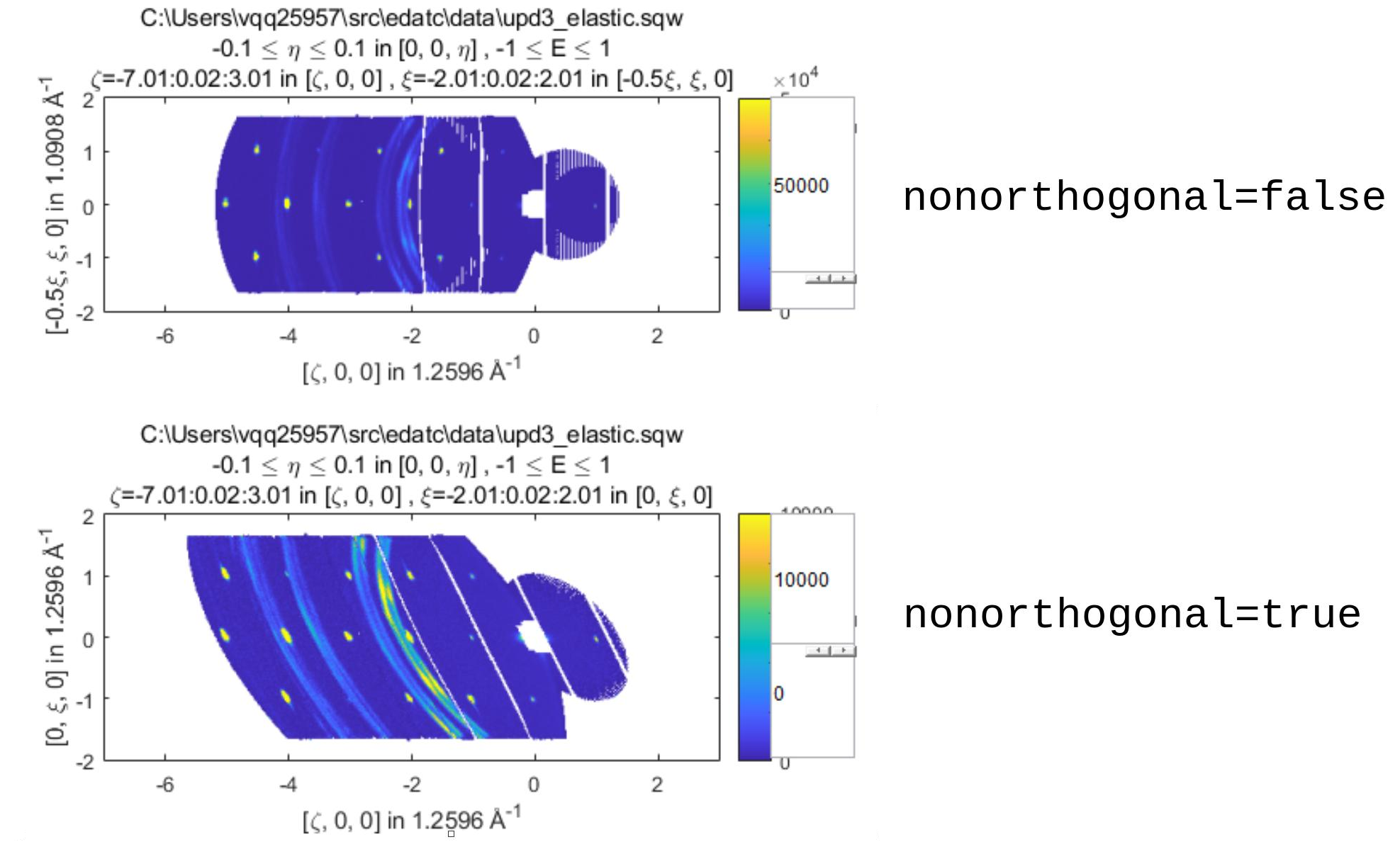
Plot to show the difference between nonorthogonal=false and nonorthogonal=true with a hexagonal material (\(\textrm{UPd}_3\)) where angdeg=[90,90,120].

We can see that for the nonorthogonal=false case, the image clearly shows the hexagonal symmetry and circular powder rings, but the axes being \([\zeta,0,0]\) and \([-0.5\xi,\xi,0]\) even in this simple case makes computing where points lie in \(hkl\) trickier.

Where we have nonorthogonal=true, this makes it easier to calculate the location of points in \(hkl\) (the Bragg peaks align in a square pattern and the axes are simply \([\zeta,0,0]\) and \([\xi,0,0]\)), but distorts the image (note the powder rings which should be circular).

5.1.5.1.2. line_proj 2D cut examples: Fe Scattering Function

Note

This dataset is available as part of the Horace source on Github.

The iron crystal has been aligned along the \([1,0,0]\) axis.

To reproduce the example below, a cut is first made along the \([0,1,0]\) and \([0,0,1]\) directions:

data_source = 'Fe_ei401.sqw';
proj = line_proj([0, 1, 0], [0, 0, 1], 'type', 'aaa');
w2 = cut(data_source, proj, [-4.5, 0.1, 14.5], [-5, 0.1, 5], [-0.1, 0.1], [-10, 10]);
plot(w2);

Note

You do not need to provide a lattice for the projection as cut will use the lattice parameters from the sqw object.

The code produces:

MAPS Fe data; reciprocal space covered by MAPS for an iron sample with incident neutron energy of 401meV.

The cut with the same parameters as above at higher energy transfer

w2 = cut(data_source, proj, [-4.5, 0.1, 14.5], [-5, 0.1, 5], [-0.1, 0.1], [50, 60]);
plot(w2);

shows clear spin waves:

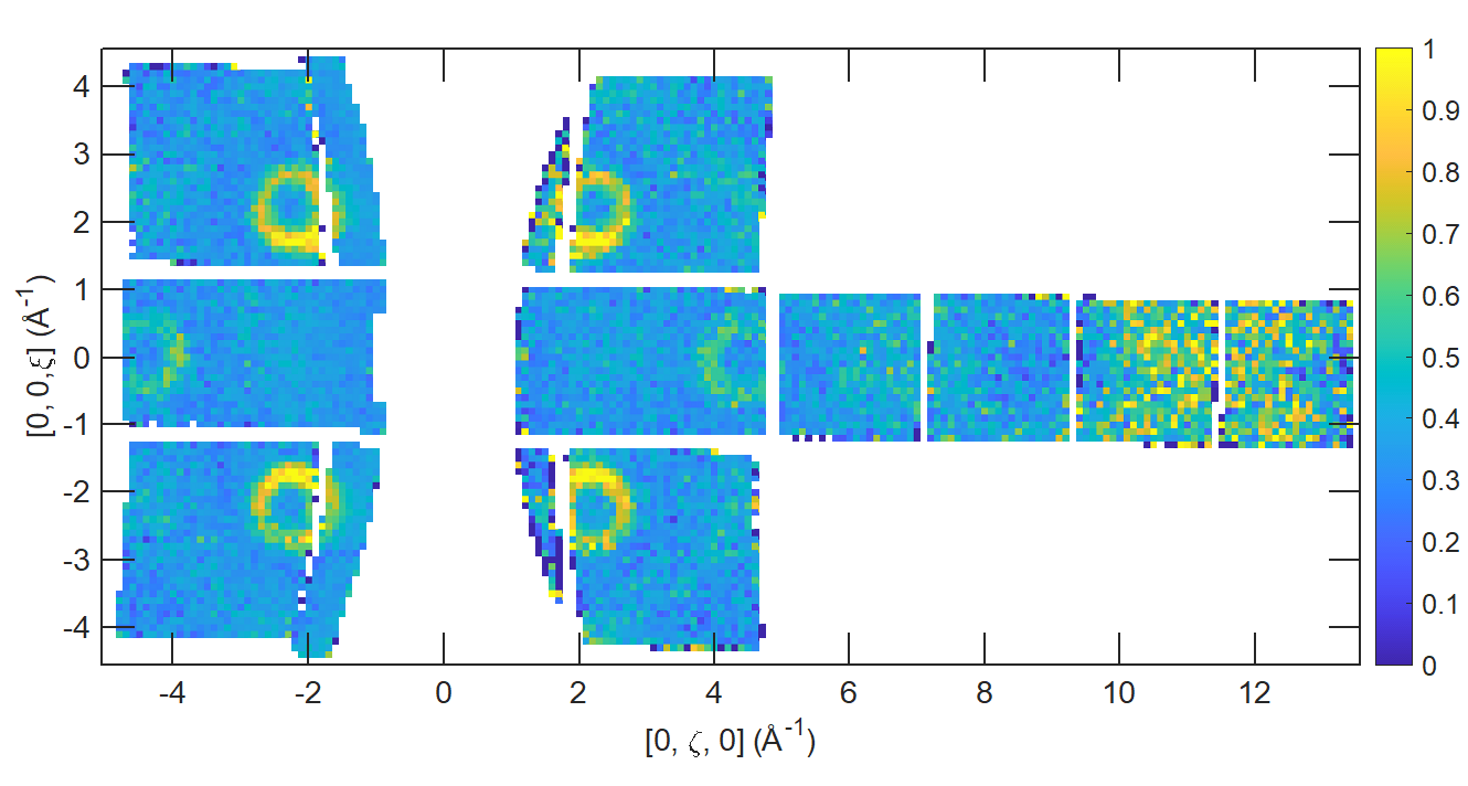
MAPS Fe Data; reciprocal space covered by MAPS for an iron sample with incident neutron energy of 401meV. Energies integrated between [50, 60].

5.1.5.1.3. line_proj 1D cut example

It is simple to take a 1-d cut by integrating over all but one axis. The example cut generated by the code below shows a cut along the \([1,1,0]\) direction (note the projection’s u & v), i.e. the diagonal of the figure above.

data_source = 'Fe_ei401.sqw';
proj = line_proj([1, 1, 0], [-1, 1, 0], 'offset', [-1, 1, 0]);
w1 = cut(data_source, proj, [-5, 0.1, 5], [-0.1, 0.1], [-0.1, 0.1], [-50, 60]);
plot(w1);

This shows the intensity of the spin wave:

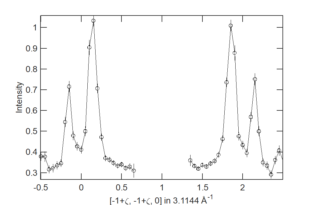
MAPS Fe Data; 1D cut along the diagonal of the 2D image above.

5.1.5.2. Spherical Projections

In order to construct a spherical projection (i.e. a projection in \(|\textbf{Q}|\), \(\theta\) (polar angle), \(\phi\) (azimuthal angle), \(E\)) we create a projection in an analogous way to the line_proj, but using the sphere_proj function.

The complete signature for sphere_proj is:

proj = sphere_proj([u][, v][, type][, alatt][, angdeg][, offset][, label][, title][, lab1][, lab2][, lab3][, lab4])

where:

• u

  The vector \(\vec{u}\) is the reciprocal space vector defining the polar-axis of the spherical coordinate system from which \(\theta\) is measured.

  See the diagram below for details.

• v

  The vector \(\vec{v}\) is the reciprocal space vector which defines the second component of the \(u\)-\(v\) plane from which \(\phi\) is measured.

  See the diagram below for details.

Note

The reciprocal space vectors \(u\)-\(v\) are not necessarily orthogonal so the actual axis from which \(\phi\) is measured lies in the plane defined by \(u\)-\(v\) vectors, orthogonal to \(u\).

Note

The \(w\) direction is not explicitly defined as part of the sphere_proj as it is always constructed to be perpendicular to the \(u\)-\(v\) plane.

Note

By default a sphere_proj will define its principal axes \(u\) and \(v\) along the \(hkl\) directions \([1,0,0]\) and \([0,1,0]\) respectively.

• type

  Three character string denoting the the projection normalization of each dimension, one character for each directions, e.g. 'add', 'arr', 'adr'.

  At the moment there is only one possible option for the first (length) component of type:

  1. 'a'

     Inverse angstroms.

  There are 2 possible options for the second and third (angular) components of type:

  1. 'd'

     Degrees

  2. 'r'

     Radians

  For example, if we wanted the \(|\textbf{Q}|\)-component to be in inverse angstroms and the angles in degrees we would have type = 'add'.

• alatt

  3-vector of lattice parameters.

• angdeg

  3-vector of lattice angles in degrees.

Note

In general, you should not need to define alatt or angdeg; by default they will be taken from the sqw object during a cut. However, there are cases where a projection object may need to be reused elsewhere.

• offset

  3-vector in \((h,k,l)\) or 4-vector in \((h,k,l,e)\) defining the origin of the projection coordinate system.

• label, etc.

  See above.

Note

If you do not provide any arguments to sphere_proj, by default it will build a sphere_proj with u=[1,0,0], v=[0,1,0], type='add' and offset=[0,0,0,0].

sp_pr = sphere_proj()

sp_pr =
   sphere_proj with properties:
          u: [1 0 0]
          v: [0 1 0]
       type: 'add'
      alatt: []
     angdeg: []
     offset: [0 0 0 0]
      label: {'|Q|'  '\theta'  '\phi'  'En'}
      title: ''

Note

Like line_proj, sphere_proj can be defined using positional or keyword arguments. However the same recommendation applies that positionals should only be used to define u and v.

sphere_proj defines a spherical coordinate system, where:

• \(|\textbf{Q}|\)

  The radius from the origin (offset) in \(hkl\)

• \(\theta\)

  The angle measured from \(\vec{u}\) to the vector (\(\vec{q}\)), which means a \(\theta\) value of \(0^{\circ}\) means that \(\vec{q}\) is parallel to \(\vec{u}\); and a \(\theta\) value of \(90^{\circ}\) means that \(\vec{q}\) is perpendicular to \(\vec{u}\).

  Mathematically this is defined as:

  \[\cos\left(\theta{}\right) = \frac{\vec{q}\cdot\vec{u}}{\left|q\right|\cdot\left|u\right|}\]

• \(\phi\)

  The angle measured between the \(u\)-\(v\) plane to the vector (\(\vec{q}\)), i.e. \(0^{\circ}\) means that \(\vec{q}\) lies in the \(u\)-\(v\) plane and \(90^{\circ}\) means that \(\vec{q}\) is normal to the \(u\)-\(v\) plane (i.e. parallel to \(w\)).

  Mathematically this is defined as:

  \[\cos\left(\phi{}\right) = \frac{\vec{p} \cdot{} \left(\vec{w} \times{} \vec{u} \right)} {\vec{q} \cdot{} \vec{w} \times{} \vec{u}}\]

  where \(\vec{p}\) is the projection of \(\vec{q}\) onto the meridian plane (the dashed line below), given by:

  \[\vec{p} = \frac{\vec{q}\cdot{}\vec{u}}{\left|u\right|^2}\vec{u}\]

• \(E\)

  The energy transfer as defined in line_proj

Note

• \(\theta\) lies in the range between \(0^{\circ}\) and \(180^{\circ}\).

• \(\phi\) lies in the range between \(-180^{\circ}\) and \(180^{\circ}\).

In radians, that is:

• \(\theta\) lies in the range between \(0\) and \(\pi\)

• \(\phi\) lies in the range between \(-\pi\) and \(\pi\).

Spherical coordinate system used by sphere_proj

Note

A spherical projection currently does not have the ability to be rescaled in \(|\textbf{Q}|\) relative to the magnitude of \(u\) or \(v\).

When it comes to cutting and plotting, we can use a sphere_proj in exactly the same way as we would a line_proj, but with one key difference. The binning arguments of cut no longer refer to \(h,k,l,E\), but to \(|\textbf{Q}|\), \(\theta\), \(\phi\), \(E\).

sp_cut = cut(w, sp_proj, Q, theta, phi, e, ...);

Warning

The form of the arguments to cut is still the same (see: Binning arguments). However:

• \(|\textbf{Q}|\) runs between \([0, \infty)\)

• \(\theta\) runs between \([0, 180]\)

• \(\phi\) runs between \([-180, 180]\)

Attempting to specify binning outside of these ranges will fail.

5.1.5.2.1. sphere_proj 2D and 1D cuts examples:

Integrating over the angular terms of a spherical projection of a single crystal dataset will give an approximation of a powder average of the sample. Integrating over the angular terms for a powder sample is a valid powder averaging.

Note

This is because (except for low scattering angles) the detectors do not cover the full \(4\pi\) solid angular range. Thus regions without detector coverage will not be sampled by the angular spherical integration.

In contrast for a true powder sample, there will be crystal grains with the correct orientation to be detected even by the limited detector coverage.

At low scattering angles (below approximately 30 degrees on LET), the detectors do cover the full angular range so the angular integration of a single crystal dataset will give a valid powder average.

These effects are important to bear in mind when modelling the scattering - e.g. for a single crystal dataset it is best to model it as a single crystal and then let Horace perform the angular integration, rather than treating it as powder data.

The following is an example using the same data as above.

data_source = 'Fe_ei401.sqw';
sp_proj = sphere_proj();
s2 = cut(data_source, sp_proj, [0, 0.1, 14], [0, 180], [-180, 180], [-10, 4, 400]);
plot(s2);

Note

Binning ranges are specified in the target coordinate system.

This script produces the following plot:

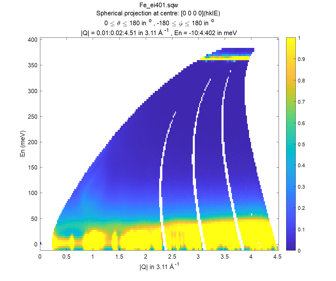
MAPS Fe data; Powder averaged scattering from iron with an incident energy of 401meV.

Note

By default, energy transfer is expressed in meV, momentum transfer \(\left|Q\right|\) in inverse Angstroms (\(Å^{-1}\)) and angles in degrees (\(^\circ\)).

This figure shows that the energies of phonon excitations are located under 50meV, some magnetic scattering is present at \(|\textbf{Q}|\) < 5 and spin waves follow the magnetic form factor.

A spherical projection allows us to investigate the details of a particular spin wave, e.g. around the scattering point \([0,-1,1]\).

data_source = 'Fe_ei401.sqw';
sp_proj = sphere_proj();
sp_proj.offset  = [0, -1, 1];
s2 = cut(data_source, sp_proj, [0, 0.1, 2], [80, 90], [-180, 4, 180], [50, 60]);
plot(s2);

The unwrapping of the intensity of the spin-wave located around \([0,-1,1]\) Bragg peak shows:

MAPS Fe data; Spin-wave scattering intensity the the origin centred about the \([0,-1,1]\) Bragg peak. A visible gap caused by missing detectors is obvious in the \(\phi\)-axis range \([-50^\circ:+50^\circ]\). Inset: Linear projection of the same region; the red lines show the approximate mapping from the linear to spherical projections.

Integrating over the whole \(\theta\) range and thus including other detectors substantially improves statistics; this is done by setting the \(\theta\) parameter to [0, 180]:

s2 = cut(data_source, sp_proj, [0, 0.1, 2], [0, 180], [-180, 4, 180], [50, 60]);

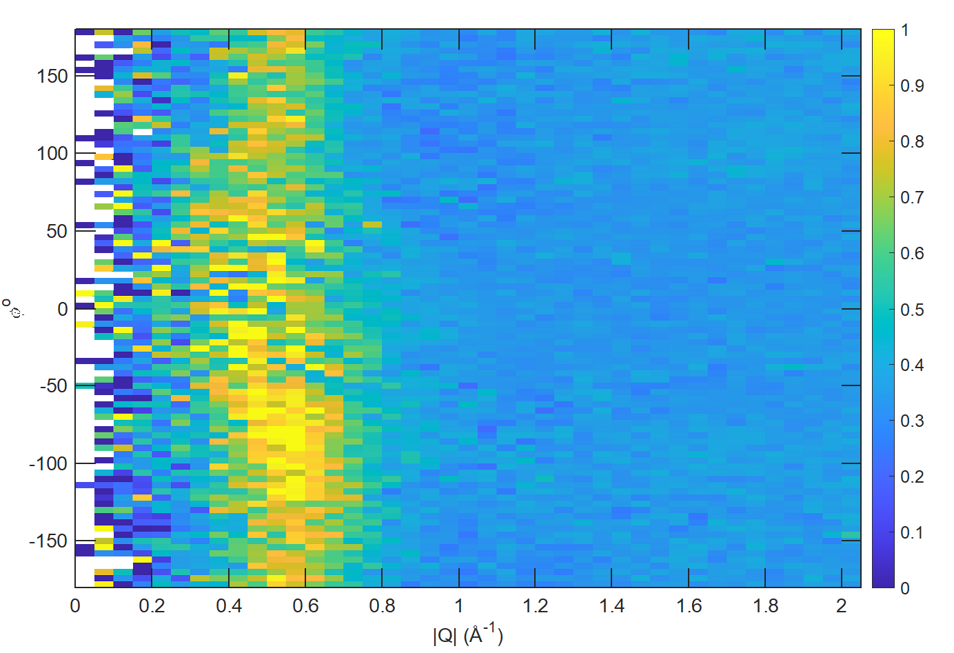
MAPS Fe data; Scattering intensity from cut averaged over all \(\theta\) spin-wave with the origin centred at the \([0,-1,1]\) Bragg peak.

The 1D cut below, generated by further integrating over the \(\phi\)-axis, shows the intensity distribution as a function of \(|\textbf{Q}|\), i.e. the distance from the spin-wave centre:

s2 = cut(data_source, sp_proj, [0, 0.1, 2], [0, 180], [-180, 180], [50, 60]);

Scattering intensity as function of distance from the scattering centre at \([0,-1,1]\).

5.1.5.3. Cylindrical Projections

In order to construct a cylindrical projection (i.e. a projection in \(\vec{q}_{\perp}\) (the radial distance from the polar axis), \(\vec{q}_{\|}\) (distance from origin along the polar axis), \(\phi\) (azimuthal angle) and \(E\)) coordinate system we create a projection in a similar way to the line_proj, but use the cylinder_proj function.

The complete signature for cylinder_proj is:

proj = cylinder_proj([u][, v][, type][, alatt][, angdeg][, offset][, label][, title][, lab1][, lab2][, lab3][, lab4])

where:

• u

  The vector \(\vec{u}\) is the reciprocal space vector defining the polar-axis of the cylindrical coordinate system along which \(\vec{q}_{\|}\) is measured.

  See the diagram below for details.

• v

  The vector \(\vec{v}\) is the reciprocal space vector which defines the second component of the \(u\)-\(v\) plane from which \(\phi\) is measured.

  See the diagram below for details.

Note

The reciprocal space vectors \(u\)-\(v\) are not necessarily orthogonal so the actual axis from which \(\phi\) is measured lies in the plane defined by \(u\)-\(v\) vectors, orthogonal to \(u\).

Note

By default a cylinder_proj will define its principal axes \(u\) and \(v\) along the \(hkl\) directions \([1,0,0]\) and \([0,1,0]\) respectively.

• type

  Three character string denoting the the projection normalization of each dimension, one character for each directions, e.g. 'aad' or 'aar'.

  At the moment there is only one possible option implemented for the length components (\(q_{\perp}\) and \(q_{\|}\)) of type:

  1. 'a'

     Inverse angstroms.

  There are 2 possible options for the third (angular) component of type:

  1. 'd'

     Degrees

  2. 'r'

     Radians

  For example, if we wanted the length components to be in inverse angstroms and the angles in degrees we would have type = 'aad'.

• alatt

  3-vector of lattice parameters.

• angdeg

  3-vector of lattice angles in degrees.

Note

In general, you should not need to define alatt or angdeg; by default they will be taken from the sqw object during a cut. However, there are cases where a projection object may need to be reused elsewhere.

• offset

  3-vector in \((h,k,l)\) or 4-vector in \((h,k,l,e)\) defining the origin of the projection coordinate system.

• label, etc.

  See above.

Note

If you do not provide any arguments to cylinder_proj, by default it will build a cylinder_proj with u=[1,0,0], v=[0,1,0], type='aad' and offset=[0,0,0,0].

cyl_pr = cylinder_proj()

cyl_pr =
   cylinder_proj with properties:
          u: [1 0 0]
          v: [0 1 0]
       type: 'aad'
      alatt: []
     angdeg: []
     offset: [0 0 0 0]
      label: {'\Q_{\perp}'  '\Q_{||}'  '\phi'  'En'}
      title: ''

Note

Like line_proj, cylinder_proj can be defined using positional or keyword arguments. However the same recommendation applies that positionals should only be used to define u and v.

cylinder_proj defines a cylindrical coordinate system, where:

• \(q_{\|}\)

  The length along the polar axis \(\vec{u}\) to \(\vec{q}\) relative to the origin (offset) in \(hkl\)

  Mathematically, this is defined as:

  \[\vec{q_{\|}} = \frac{\left(\vec{q} \cdot{} \vec{u}\right)} {\left|u\right|} \vec{u}\]
  \[q_{\|} = \left| \vec{q_{\|}} \right|\]

• \(q_{\perp}\)

  The radial distance from the polar axis \(\vec{u}\) to \(\vec{q}\) relative to the origin (offset) in \(hkl\).

  Mathematically, this is defined as:

  \[\vec{q_{\perp}} = \vec{q} - \vec{q_{\|}}\]
  \[q_{\perp} = \left| \vec{q_{\perp}} \right|\]

• \(\phi\)

  The angle measured between the \(u\)-\(v\) plane to the vector (\(\vec{q}\)), i.e. \(0^{\circ}\) lies in the \(u\)-\(v\) plane and \(90^{\circ}\) is normal to the \(u\)-\(v\) plane (i.e. parallel to \(\vec{w}\)).

  Mathematically this is defined as:

  \[\cos\left(\phi{}\right) = \frac{\vec{q_{\perp}} \cdot \left(\vec{w} \times \vec{u}\right)} {\left|\vec{q_{\perp}}\right|\left|\vec{u}\right|\left|\vec{w}\right|}\]

• \(E\) is the energy transfer as defined in line_proj

Note

\(\phi\) lies in the range between \(-180^{\circ}\) and \(180^{\circ}\). The cylinder_proj settings allow to change these values to radians so \(-\pi \leq \phi \leq \pi\).

Cylindrical coordinate system used by cylinder_proj

Note

A cylindrical projection currently does not have the ability to be rescaled in \(Q_{\perp}\) or \(Q_{||}\) relative to the magnitude of \(u\) or \(v\) vectors.

When it comes to cutting and plotting, we can use a cylinder_proj in exactly the same way as we would a line_proj, but with one key difference. The binning arguments of cut no longer refer to \(h,k,l,E\), but to \(q_{\perp}\), \(q_{\|}\), \(\phi\), \(E\) variables.

sp_cut = cut(w, cylinder_proj, Q_\perp, Q_||, phi, e, ...);

Warning

The form of the arguments to cut is still the same (see: Binning arguments). However:

• \(q_{\perp}\) runs between \([0, \infty)\)

• \(\phi\) runs between \([-180, 180]\)

requesting binning outside of these ranges will fail.

5.1.5.3.1. cylinder_proj 2D and 1D cuts examples:

Cylindrical projection can be used to obtain cylindrical cuts in a manner analogous to linear and spherical projections.

The main use of cylindrical projection is for cuts with axis parallel to the incident beam as background scattering in inelastic instruments often has cylindrical symmetry.

Taking the previously used dataset and using the code:

data_source = 'Fe_ei401.sqw';
cyl_proj = cylinder_proj();

%% A

w2_Qtr_dE = cut(data_source, cyl_proj, [0, 0.1, 14], [-4, 4], [-180, 180], [-10, 4, 400]);
plot(w2_Qtr_dE);
keep_figure;

%% B

w2_Qtr_Qll = cut(data_source, cyl_proj, [0, 0.1, 14], [-4,0.1,4], [-180, 180], [50, 60]);
plot(w2_Qtr_Qll);
keep_figure;

%% C

w2_Qtr_phi = cut(data_source, cyl_proj, [0, 0.1, 14], [-4,,4], [-180,2,180], [50, 60]);
plot(w2_Qtr_phi);

one can easily obtain various cuts taken along different coordinate axes.

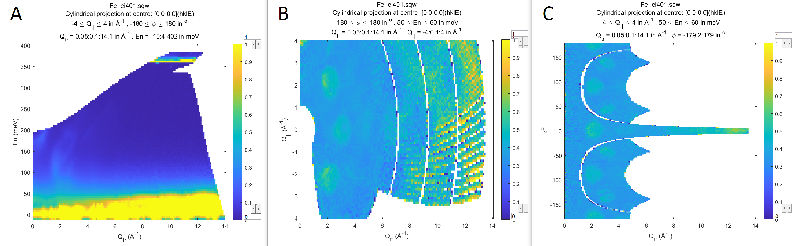
Cylindrical cuts along different coordinate axes

It is also possible to make one dimensional cylindrical cuts. The following code creates a plot which shows the behaviour of the scattering intensity as a function of \(Q_{\perp}\) at different \(Q_{||}\):

data_source ='Fe_ei401.sqw';
cyl_proj = cylinder_proj();
n_cuts = 2;
w1 = repmat(sqw,1,n_cuts);
colors = 'krgb';
symbols = '.+*x';
for i=1:n_cuts
    cut_center = -4+(i-1)*(8/n_cuts);
    Qll_range = [cut_center-0.1,cut_center+0.1];
    w1(i) = cut(data_source, cyl_proj, [0, 0.1, 14], Qll_range, [-180,180], [50,60],'-nopix');
    acolor(colors(i));
    amark(symbols(i));
    pd(w1(i))
end
legend('Q_{||}=-4','Q_{||}=-2','Q_{||}=0','Q_{||}=2');

Cylindrical cuts along \(Q_{\perp}\)

Note

The script above lets you take up to 4 cuts by changing n_cuts, here we present just two for clarify.

5.1.6. Additional notes

Note

The number of binning arguments need only match the dimensionality of the object w (i.e. the number of plot axes), so can be fewer than 4.

Note

You cannot change the binning in a dnd object, i.e. you can only set the integration ranges, and have to use [] for the plot axis. The only option you have is to change the range of the plot axis by specifying [lo1,0,hi1] instead of [] (the ‘0’ means ‘use existing bin size’).

5.1.6.1. Changing Projections

When a cut will change projections (i.e. the source projection type is different or the principal-axes are not orthogonal to the target projection) there are a few things to be aware of, particularly when you specify automatic ([], [step]) binning arguments.

Binning range meaning

When you specify the binning ranges these are defined in the the “target” (desired) coordinate system. E.g. in cutting from a linear to a spherical projection, the meanings are:

x = sqw(..) % in linear projection
y = cut(x, sphere_proj(), **R**, **THETA**, **PHI**, **E**, ..)

Automatic Binning Arguments

If you provide automatic binning arguments, an algorithm will attempt to create the minimum bounding shape in the new projection that entirely encapsulates the source projection. The parameters from this bounding shape will then be substituted into the places where automatic binning arguments are requested.

Warning

This algorithm will not change the number of bins unless the [step] form is used, but will change the ranges and thus the size of the bins in this instance.

If you do not specify a step, ensure you have checked that the binning is suitable in the new projection, or you may waste time having to re-cut your dataset.

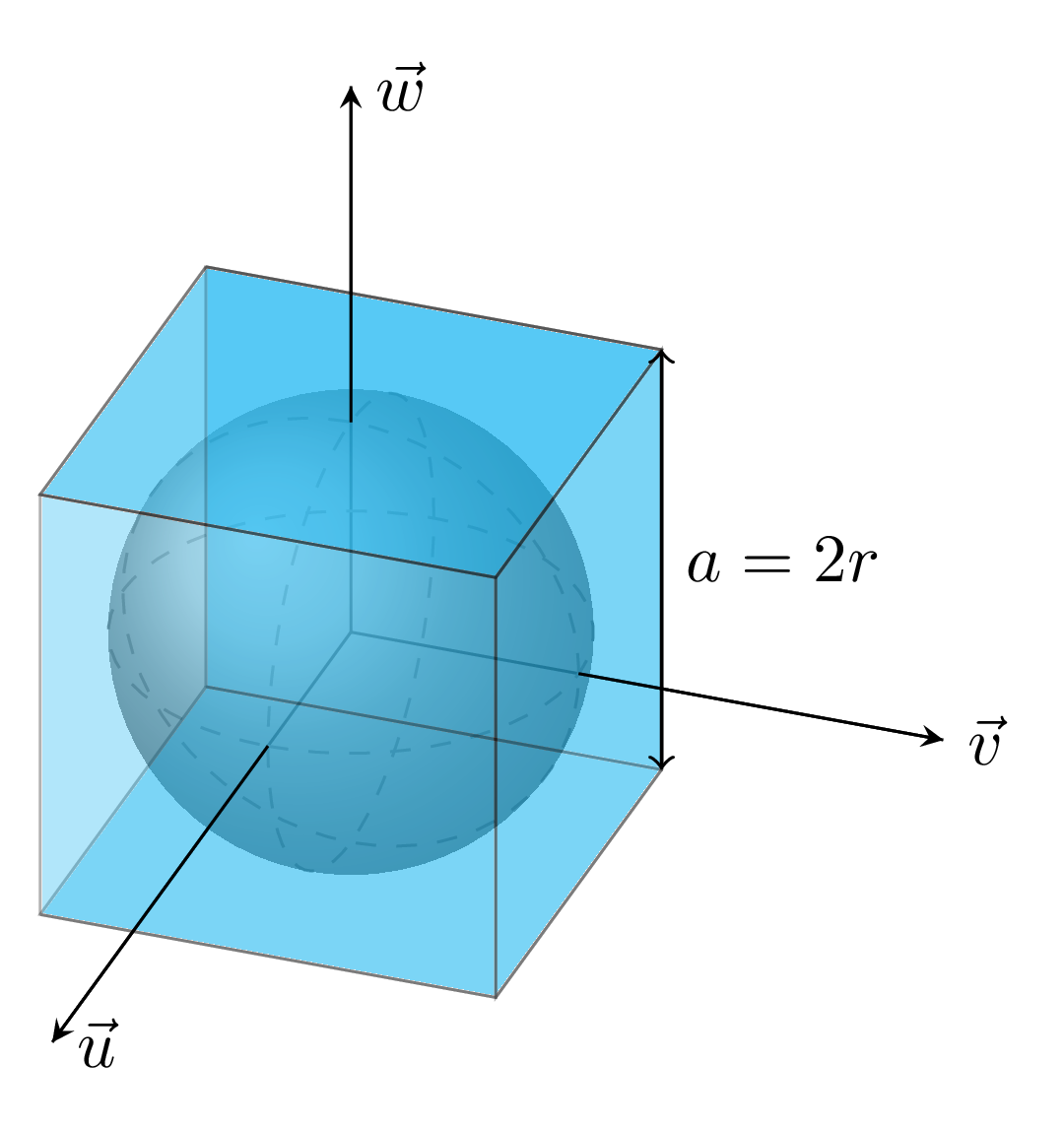
Example showing a linear projection (target) encapsulating a spherical projection (source). Here, if we consider a sphere of radius \(r\), then the encapsulating cuboid has sidelength (\(a\)) of size \(2r\).

Example

If:

• you provide an empty binning range ([]) as the third binning argument in your cut and,

• your source coordinate system is linear and,

• the target coordinate system is cylindrical, then:

the cut algorithm will try to compute the \(\phi\) range (the 3^rd coordinate of the cylindrical projection) which encapsulates the source cuboid in the target (cylindrical) coordinate system.

The number of bins in \(\phi\) will be equal to the number of bins in the 3^rd dimension (\(\vec{w}\)) of the source projection. If the 3^rd dimension of the source projection was an integration axis, the \(\phi\) of the target projection will also be an integration axis; if it was a plot axis, it will likewise remain a plot axis in the target projection, as expected.

Warning

In contrast to cutting without a projection change, when changing projections [] and [0] have different meanings.

• [] will take the number of bins in the source dimension

• [0] will take the step length in the source dimension

Cutting with [0] may lead to strange or incorrect results when changing projections. E.g. a q-step of 0.01 may be reasonable in a linear projection, but when transformed to a spherical or cylindrical projection it may be used as the step size for the \(\phi\) binning range (-180:180 ), creating 36000 bins in \(\phi\) direction, which may be problematic.

Warning

The algorithm which identifies binning ranges is just a simple algorithm.

While it works reliably in simple cases, e.g. for transformations described by projections of the same kind (e.g. sphere_proj->sphere_proj), where the offset between the two projections is unchanged. In more complex cases (e.g. line_proj->cylinder_proj or where the polar-axis of the cylindrical projection is not aligned with any of the line_proj axes), the algorithm may not converge quickly. After a number of failed iterations, it will give up and issue a warning which looks like:

' target range search algorithm have not converged after 5 iterations.
  Search have identified the following default range:
 0        0.0120  -179.9641
 1.5843   90.0000  179.9641
 This range may be inaccurate'

The user must evaluate how acceptable this result is for the desired cut and if in doubt, specify the binning arguments manually to get their desired binning.

5.1.7. Legacy calls to cut: cut_sqw and cut_dnd

Historically, cut came in two different forms cut_sqw and cut_dnd. These forms are still available now, however their uses are more limited and mostly discouraged.

• cut_sqw is fully equivalent to cut except that attempting to apply it to a dnd object or file, will raise an error.

• cut_dnd is equivalent to cut except it only ever returns a dnd as though -nopix had been passed.

5.2. section

section is an sqw method, which works like cut, but uses the existing bins of an sqw object rather than rebinning.

wout = section(w, p1_bin, p2_bin, p3_bin, p4_bin)

Because it only extracts existing bins (and their pixels), this means that it doesn’t need to recompute any statistics related to the object itself and is therefore faster and more efficient. However, it has the limitation that it cannot alter the projection or binning widths from the original.

The parameters of section are as follows:

• w

  The array of sqw object(s) to be sectioned.

• pN_bin

  The range of bins specified as bin edges to extract from w.

  There are three valid forms for any pN_bin:

  • [], [0]

    Use the original binning.

  • [lo, hi]

    Take a section of original axis which lies between lo and hi values. The range of the resulting image in this case is the range between left edge of image bin containing lo value and right edge of bin containing hi value.

Note

The size of pN_bin must match the dimensionality of the underlying dnd object.

Note

These parameters are specified by inclusive edge limits. Any ranges beyond the the sqw object’s img_range will be reduced to only capture existing bins.

Warning

The bins selected will be those whose bin centres lie within the range lo - hi, this means that the actual returned img_range may not match [lo hi]. For example, a bin from 0 - 1 (centre 0.5) will be included by the following section despite the bin not being entirely contained within the range. The resulting image range will be [0 1].

section(w, [0.4 1])

In order to extract bins whose centres lie in the range [-5 5] from a 4-D sqw object:

w4_red = section(w4, [-5 5], [], [], [])