13. Plotting
An exhaustive list of commands to do with plotting your data - one of the primary functions of Horace!
13.1. plot
Plot a dnd or sqw object. In general the axes are the dimensions of the
dnd or sqw objects themselves according to the cut and the
signal/intensity.
For 1-dimensional objects a series of markers with errorbars are connected by a line.
For 2-dimensional objects a 2D colourmap is displayed.
For a 3-dimensional object the
sliceomaticprogram is used, where a series of 2D slices within a box are plotted.
Warning
This does not work for 0-dimensional objects (single points), or 4-dimensional objects (we couldn’t think of a way of displaying 4 dimensions plus intensity!).
plot(w)

[figureHandle_, axesHandle_, plotHandle_] = plot(w)
The second line of code (with outputs) returns Matlab handles to the figure window, the axes, and the plot respectively. These are useful if, for example, you wish to resize the axes, change the font size of labels, etc.
13.2. smooth
wsmooth = smooth(w)

wsmooth = smooth(w, [wid_x, wid_y, ..], shape)
smooth allows you to smooth the data for plotting. You can optionally
specify the width and smoothing function ('hat' or 'gaussian'). The
defaults are 'hat', and 3 bins either side in all directions.
Note
You can only apply smoothing to dnd objects, not to sqw objects,
since with the latter you would have to destroy the pixel information that
the object is designed to hold. To convert an sqw object (win) to a
dnd, simply type wout = dnd(win).
13.2.1. Altering plot characteristics and other useful commands
13.3. Colour of lines and markers
To change the marker and line colour in a 1-dimensional Horace plot, type
acolor <the color that you want>
e.g. for a red plot:
acolor red
13.4. Line style
To change the line style in a 1-dimensional plot, type e.g.
aline --
to make a dashed line. You can also change the line thickness with something like
aline 2
To change multiple characteristics, type e.g.
aline(2,'--')
Type help aline in Matlab for a full list of options.
13.5. Marker style
You can change the style of marker in a 1-dimensional plot in a similar way to the above, e.g.
amark o %gives a circular marker
amark 6 %sets marker size to 6
amark(6,'o') %sets a circular marker with size 6
Type help amark in Matlab for a full list of options.
13.6. Axes Limits
To change the x, y, or z limits of a plot, type e.g.
lx 0 3
ly -6 1
lz -2 2
which sets the x-axis limits to be 0 to 3, the y-axis limits to be -6 to 1, and
the z-axis limits to be -2 to 2. Note the lz is used to change the color
scale on a colormap plot.
To set the range to cover the full data range, just issue the commands without a range:
lx
ly
lz
You can also change the axes scales to be linear or logarithmic using
- ::
linx logx
liny logy …
13.7. Cursor
In order to get a cursor on your Horace plots, type
xycursor
You then left click the mouse on a position in a figure, and the x and y values are printed in the Matlab window. You can do this multiple times. To turn off the cursor, hit the carriage return key.
Alternatively, to use a cursor to click to select x and y values and print them in the Matlab command window or save them to arrays, type
xyselect

[x, y] = xyselect
13.8. Keeping plots
To store a figure in your current session (i.e. so that the next plot you make opens in a new window, with the current plot preserved), type
keep_figure
If you have multiple figures open and you wish to alter one of them (e.g. by appending a line or more data to it) that has been kept using the above command, click on it and then type
make_current
Note that both of these options are also available in drop-down menus in the figures windows themselves.
13.8.1. One dimensional plots
In the following the object being plotted can be a single sqw or dnd object, or an array of objects.
13.9. dd (draw data)
Plotting command for 1-dimensional objects only, plotting markers, errorbars, and connecting lines. Any existing 1-dimensional figure window is cleared before plotting i.e. existing data is not overplotted. If you use this command and the current figure window does not correspond to a 1-dimensional object, then a new figure window will be created.
dd(w_1d)

[figureHandle_, axesHandle_, plotHandle_] =  dd(w_1d)
13.10. dl (draw line)
Plot line between points for a 1-dimensional object. No markers or errorbars displayed.
dl(w_1d)

[figureHandle_, axesHandle_, plotHandle_] = dl(w_1d)
13.11. dm (draw markers)
Plot markers at points for a 1-dimensional object. No line or errorbars displayed.
dm(w_1d)

[figureHandle_, axesHandle_, plotHandle_] = dm(w_1d)
13.12. dp (draw points)
Plot markers and errorbars for a 1-dimensional object. No lines linking points are displayed.
dp(w_1d)

[figureHandle_, axesHandle_, plotHandle_] = dp(w_1d)
13.13. de (draw errors)
Plot errorbars at points for a 1-dimensional object. No linking lines or markers are displayed.
de(w_1d)

[figureHandle_, axesHandle_, plotHandle_] = de(w_1d)
13.14. dh (draw histogram)
Plot histogram of a 1-dimensional object.
dh(w_1d);

[figureHandle_, axesHandle_, plotHandle_] = dh(w_1d)
13.15. pd (plot data)
Overplotting command for 1-dimensional objects only, plotting markers, errorbars, and connecting lines.
If the current window is a 1-dimensional figure window the existing plot is overplotted.
If there is no current figure window then it plots a new one.
If you use this command and the current figure window does not correspond to a 1-dimensional object, then a new figure window will also be created.
pd(w_1d)

[figureHandle_, axesHandle_, plotHandle_] =  pd(w_1d)
13.16. pl (plot line)
Overplot line between points for a 1-dimensional object. No markers or errorbars displayed.
pl(w_1d)

[figureHandle_, axesHandle_, plotHandle_] = pl(w_1d)
13.17. pm (plot markers)
Overplot markers at points for a 1-dimensional object. No line or errorbars displayed.
pm(w_1d)

[figureHandle_, axesHandle_, plotHandle_] = pm(w_1d)
13.18. pp (plot points)
Overplot markers and errorbars for a 1-dimensional object. No lines linking points are displayed.
pp(w_1d)

[figureHandle_, axesHandle_, plotHandle_] = pp(w_1d)
13.19. pe (plot errors)
Overplot errorbars at points for a 1-dimensional object. No linking lines or markers are displayed.
pe(w_1d)

[figureHandle_, axesHandle_, plotHandle_] = pe(w_1d)
13.20. ph (plot histogram)
Overplot histogram of a 1-dimensional object.
ph(w_1d);

[figureHandle_, axesHandle_, plotHandle_] = ph(w_1d)
13.21. ploc (plot line over current)
Overplot a line in the current figure, regardless of type (i.e. can plot a 1d curve on top of a 2d dataset, such as when plotting a dispersion relation over a 2d Q-E slice).
ploc(w_1d);
13.22. pdoc (plot data over current)
Overplot line, markers and error bars in the current figure, regardless of type.
pdoc(w_1d);
13.23. pmoc (plot markers over current)
Overplot markers in the current figure, regardless of type.
pmoc(w_1d);
13.24. ppoc (plot points over current)
Overplot markers and error bars in the current figure, regardless of type.
pm
ppoc(w_1d);
13.25. peoc (plot errors over current)
Overplot error bars in the current figure, regardless of type.
peoc(w_1d);
13.26. phoc
Overplot a histogram in the current figure, regardless of type.
phoc(w_1d);
13.26.1. Two dimensional plots
13.27. da (draw area)
Area plot for a two-dimensional object, with colour-scale signifying
intensity. It is this that is called when plot is used for a 2-dimensional
object.
da(w_2d);

[figureHandle_, axesHandle_, plotHandle_] = da(w_2d)
13.28. ds (draw surface)
Surface plot for a two-dimensional object, with colour scale and contour signifying intensity.
ds(w_2d);

[figureHandle_, axesHandle_, plotHandle_] = ds(w_2d)
13.29. ds2 (draw surface from 2 sources)
This routine is especially useful for making surface plots of dispersion relations when used in conjunction with dispersion.
Make a surface plot of a 2D sqw or d2d object, with the signal array
defining the contours and the error array (or another data source) providing the
intensity.
ds2(w_2d)       % Use error bars to set colour scale

ds2(w_2d,wc_2d) % Signal in wc sets colour scale (sqw or d2d object with same array size as w, or a numeric array)
This differs from ds in that the signal sets the z-axis, and the colouring
is set by the error bars, or another object. This enables a function of three
variables to be plotted (e.g. dispersion relation where the ‘signal’ array holds
the energy and the error array holds the spectral weight).
One can optionally return figure, axes and plot handles:
[fig_handle, axes_handle, plot_handle] = ds2(w_2d,...)
13.30. pa (plot area)
Overplot an area plot of a two-dimensional object
pa(w)
Optionally return figure, axes and plot handles:
[fig_handle, axes_handle, plot_handle] = pa(w)
13.31. ps (plot surface)
Overplot a surface plot of a two-dimensional object
ps(w_2d)
Optionally return figure, axes and plot handles:
[fig_handle, axes_handle, plot_handle] = ps(w_2d)
13.32. ps2 (plot surface from 2 objects)
Overplot a surface plot of a two-dimensional object with the colour scale set by the error bars or a second object)
ps2(w_2d)

ps2(w_2d, wc_2d)
Optionally return figure, axes and plot handles:
[fig_handle, axes_handle, plot_handle] = ps2(w_2d,...)
13.33. spaghetti_plot
Plots data in sqw HKL directions.
>>wsp = spaghetti_plot([0 0 0; 0.5 0.5 0.5; 0.5 0.5 0],sqw_file,'labels',{'\\Gamma','R','M'}); % made spaghetti plot
>>wsp = spaghetti_plot(plot_data); % plot existing spaghetti plot data
where:
rlp – Array of reciprocal lattice points e.g. [0,0,0; 0,0,1; 1,0,1; 1,0,0],
data_source – either sqw object or filename of a file with sqw-type data
(character string or cellarray with one character string) or, array of d2d objects representing
spaghetti plot panels. In this case, rlp points are optional and can be fully replaced by labels.
The program works as if rlp option is missing.
wdisp – Array of d2d or IX_dataset_2d objects containing the cuts -
e.g. previous generated spaghetti plot.
call help spaghetti_plot for extensive set of optional keyword options (can be abbreviated to single letter).
An example of the plot, produced py shaghetti_plot routine is presented on the following picture:
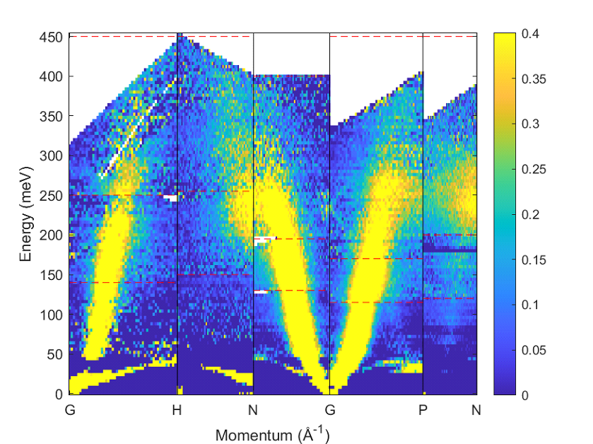
Fig. 13.1 Spaghetti plot example
13.33.1. Three dimensional plots
13.34. sliceomatic
Sliceomatic plot of multiple area plots, for a 3-dimensional object. This
function is called by the plot routine.
sliceomatic(w_3d);
13.35. sliceomatic_overview
As sliceomatic, but the default view is from above. In effect this means you
see a 2d slice which can be animated/changed by the third slider bar. Useful for
e.g. following a spin wave dispersion ring/cone as a function of energy.
sliceomatic_overview(w_3d);               % views down the third projection axis by default

sliceomatic_overview(w_3d, axis_number);  % view down the given axis number (axis_number = 1,2 or 3)
13.36. Miscellaneous functions
meta(fig)allows you to copy the figure into a metafile. On Windows, this function puts the file in the clipboard so that it can be pasted directly into Word, Powerpoint etc.genieplotis a singleton, which describes common settings (configuration) used in Horace plots.genieplot.instance()gives access to the settings common to all Horace figures. The result behaves similarly to the properties of MATLABfigureclasses, but is applied for all figures plotted after the change.See Global settings for Horace graphics: genieplot to get more details about Horace graphics configurations.
src(fig). If you plotted an object and want to return the object, used as the source of the figure, you may usesrccommand:
>>source = src(fig);
or
>>source = src(figure_number);
This command returns you the Horace object (sqw, dnd or IX_dataset_nD) used as the source of the plot. The option to store references to plotted objects in figure
handles is configured by Horace Configuration Settings property
store_src_in_plots. If your machine has very limited memory, you may want set this property to false so this option becomes unavailable and you may delete your resulting
objects immediately after they were plotted. By default, reference to plotted Horace object is stored in figure handle’s UserData property, so the source object exist until its figure exists. src command finds appropriate figure handle and returns contents of UserData property.
draw_mask. The algorithm allows you to define mask by drawing it on plotted image if image processing toolbox is installed. See draw_mask for more details about this routine.