3. Data diagnostics

Horace contains various tools for diagnosing issues with the data. The foremost of these is the run_inspector tool.

If you wish to decompose an sqw object into the data from its constituent runs, the split routine outlined below can be used. If necessary after manipulation, these data can then be recombined using the join routine.

3.1. run_inspector

The run_inspector routine may be used on 1d or 2d sqw objects to plot the data from each individual run.

run_inspector(w)

run_inspector(w,'ax',[-5,4,0,370])

run_inspector(w,'ax',[-5,4,0,370],'col',[0,1])

The 'ax' and 'col' arguments allow you to specify the xy axes, and the colour scale, of the resulting plots. If these options are not set then each frame will be plotted with different (tight) axes and a different colour scale.

To toggle through the frames, there are several keyboard options:

• Enter (Return) - play/pause video (5 frames-per-second default).

• Backspace - play/pause video a factor 5 slower.

• Right/left arrow keys - advance/go back one frame.

• Page down/page up - advance/go back 10 frames.

• Home/end - go to first/last frame of video.

Let us illustrate the information that may be obtained by means of an example. First we generate a QE slice such as the one below

Selected QE slice

We can now use run_inspector to plot a series of slices that come from a single contributing dataset, shown below.

Frame 1 in run inspector

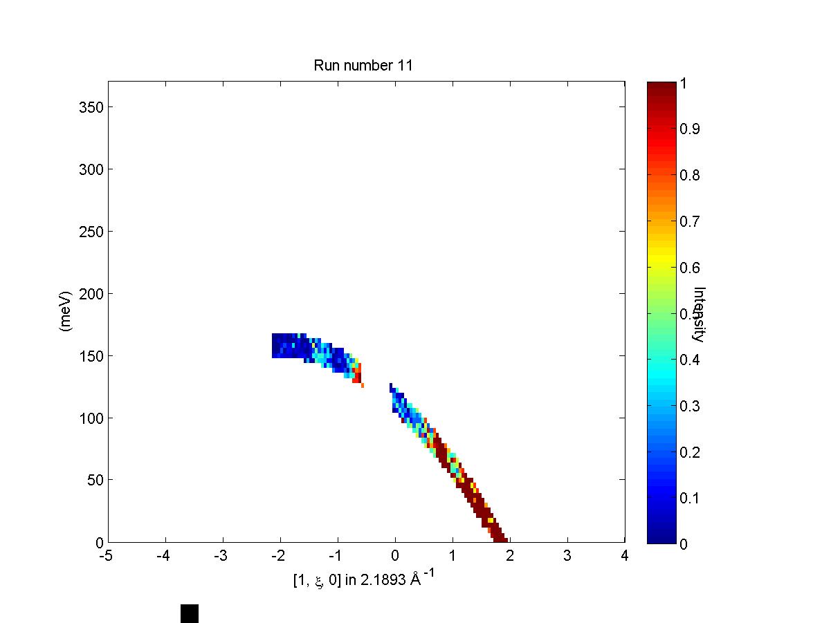
Frame 11 in run inspector

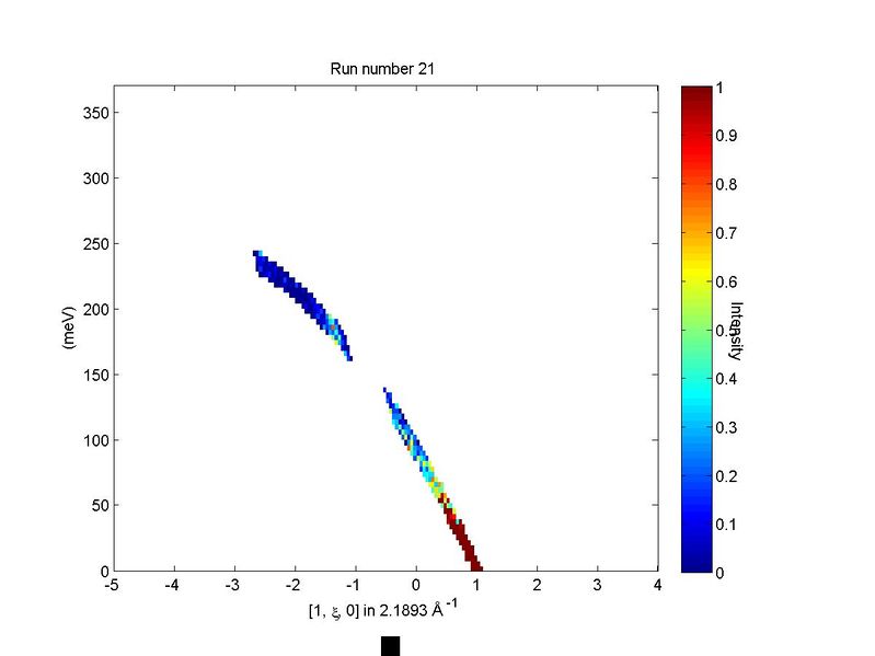
Frame 21 in run inspector

3.2. split

Split an sqw object into an array of sqw objects, each containing data from a single contributing run. So if your dataset comprises information from 100 runs, the output will be a 100-by-1 array of sqw objects.

wout = split(w)

The inputs are:

w - an sqw object.

The output is:

wout - an array of sqw objects, each one made from a single .spe data file

3.3. join

Inverse of split - takes an array of sqw objects that have been created using split and recombines them.

wout = join(w[, wi])

The inputs are:

w - an array of sqw objects, each one made from a single .spe data file

wi [Optional] - the original pre-split sqw object (recommended).

The output is:

wout - an sqw object formed of from the w input.

3.4. Instrument view cut

Normally Horace works with \(S(\vec{Q},\omega)\) scattering function build in reciprocal coordinate system related to a crystal. If sample is not sufficiently large to allow neutrons thermalization or instrument have various problems with its detectors or background scattering, some scattering artefacts may add noise or unrelated signals to measured \(S(\vec{Q},\omega)\) function. These artefacts will have spherical symmetry around the beam direction. To clearly identify such artefacts one may use instrument_view_cut algorithm:

wout = instrument_view_cut(sqw_source,[0,theta_step,theta_max],[En_min,En_step,En_max]);

Where sqw_source is an source sqw object with pixels, and two other arguments define binning in two directions. theta – the angle between beam and detector directions and En are the energy transfer values. The algorithm makes the cut in the spherical coordinate system wich z-axis is aligned along the beam direction. According to Horace agreement, beam in Horace is directed along \(e_{x}\) coordinate or direction \(\vec{u}\) of the crystal (see Chapter on Generating SQW files for details):

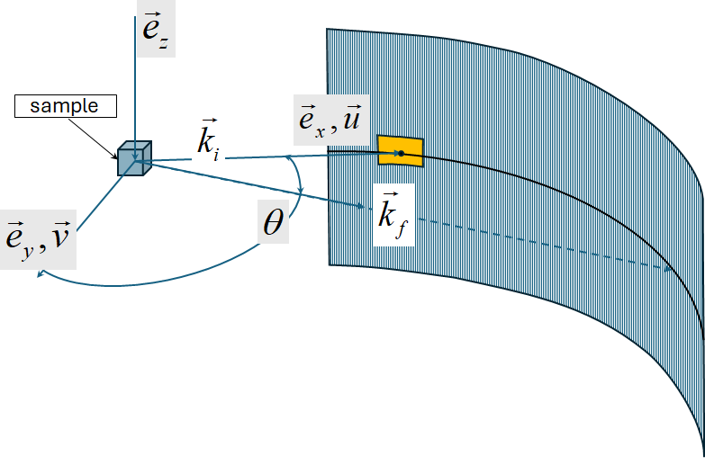
Spherical coordinate system aligned with the beam and used by instrument_view_cut.

The algorithm processes whole sqw source so takes a while to complete. Picture below shows the result of executing this algorithm on two old (2010) MAPS sqw files produced without diagnostics running over contributing nxspe files. There are various instrument artefacts clearly observable on the images. The noisy ADC are not even identifiable by diagnostics.

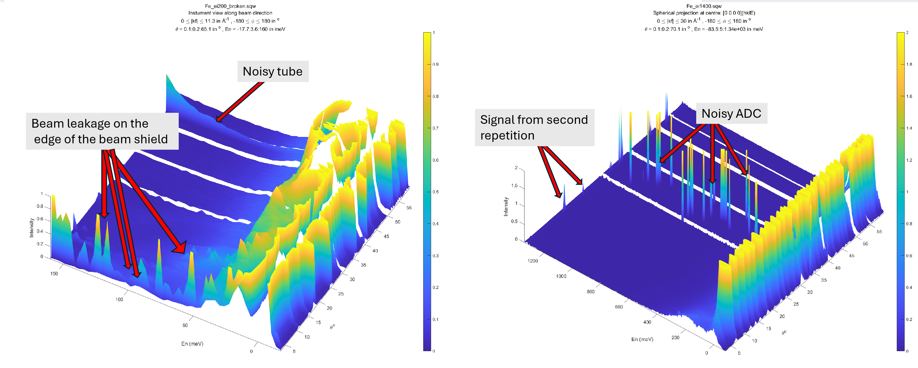
Various issues identified on instrument view.

The best way of dealing with these kind of issues if they can not be clearly observable from a single run is to use Mantid to add together all workspaces intended to use as Horace source data, display them on Mantid instrument view and create hard mask there.

There is another issue which can be identified by this algorithm usually while diagnosing old sqw data, as this issue have been hopefully fully fixed in Horace-4. You may notice, that cut applied over the whole sqw file range suddenly start loosing substantial fraction of pixels. For example, normal cut log for a cut applied over whole sqw file range will look like:

*** Cutting file-backed sqw object; returning result in file –> ignored as cut contains no pixels

*** Step 1 of 196; Read data for 20000000 pixels – processing data… —–> included 20000000 pixels

*** Step 2 of 196; Read data for 20000000 pixels – processing data… —–> included 20000000 pixels

*** Step 3 of 196; Read data for 20000000 pixels – processing data… —–> included 20000000 pixels

*** Step 4 of 196; Read data for 20000000 pixels – processing data… —–> included 20000000 pixels

*** Step 5 of 196; Read data for 20000000 pixels – processing data… —–> included 20000000 pixels

*** Step 6 of 196; Read data for 20000000 pixels – processing data… —–> included 20000000 pixels

*** Step 7 of 196; Read data for 20000000 pixels – processing data… —–> included 20000000 pixels

*** Step 8 of 196; Read data for 20000000 pixels – processing data… —–> included 20000000 pixels

*** Step 9 of 196; Read data for 20000000 pixels – processing data… —–> included 20000000 pixels

....

Sometimes running cut on old Horace data, despite making instrument_view_cut over whole instrument ranges will produce log which look like:

*** Cutting file-backed sqw object; returning result in file –> ignored as cut contains no pixels

*** Step 1 of 264; Read data for 20000000 pixels – processing data… —–> included 5162352 pixels

*** Step 2 of 264; Read data for 20000000 pixels – processing data… —–> included 10791836 pixels

*** Step 3 of 264; Read data for 20000000 pixels – processing data… —–> included 5338109 pixels

*** Step 4 of 264; Read data for 20000000 pixels – processing data… —–> included 0 pixels

*** Step 5 of 264; Read data for 20000000 pixels – processing data… —–> included 0 pixels

*** Step 6 of 264; Read data for 20000000 pixels – processing data… —–> included 191651 pixels

*** Step 7 of 264; Read data for 20000000 pixels – processing data… —–> included 7974898 pixels

*** Step 8 of 264; Read data for 20000000 pixels – processing data… —–> included 12112223 pixels

*** Step 9 of 264; Read data for 20000000 pixels – processing data… —–> included 1943239 pixels

....

despite the cut is performed over whole instrument ranges. This indicates subtle issue in Horace sqw files, where they lost synchronization between pixels information and information about crystal orientation. To clarify this issue exactly, one may run instrument_view_cut with -check_correspondence option.

wout = instrument_view_cut(source_sqw,[0,0.2,140],[],'-check_correspondence');
plot(wout)

This option force 2D cut in \(|k_{f}|\) - \(dE\) coordinates. As these values are connected by arithmetic relationship, the cut in these coordinates should represent a line. If one see a 2-dimensional image instead, the correspondence between pixel information describing neutron “pseudo-events” and experiment information describing runs and crystal orientation is violated. The following figure represents two sqw datasets, where the first one was build with correct correspondence between experiment and pixels information and the second one – where this correspondence have been broken.

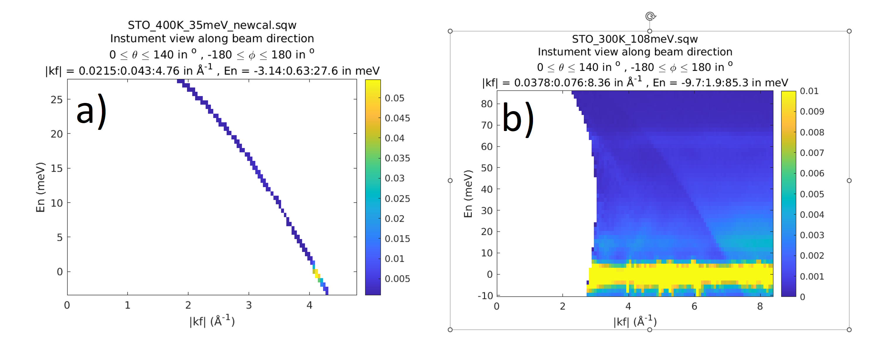
Correct – a) and broken – b) relationship between experiment information and pixels information.

The dataset with broken pixel-experiment correspondence can be cut, sliced and multifitted, but Tobyfit would not produce correct result on it. To use Tobyfit, one needs to rebuild such sqw dataser using Horace-4. If you do not have original data to reproduce such sqw dataset and need to use Tobyfit, contact HoraceHelp@stfc.ac.uk. The team should be able to help you rebuilding such sqw dataset.