Getting started

In order to get going with Horace we suggest that you take a little time to familiarise yourself with the program. To aid this we have created the following step-by-step guide that takes you through the process of converting SPE files into a format useable by Horace, and then shows you how to do different kinds of plot, how to manipulate your data, and finally how to simulate and fit your data. To do this we will refer to the demonstration files included in

C:\\mprogs\\Horace\\demo\\

which relate to a real experiment to investigate spin excitations in Fe using the MAPS spectrometer at ISIS.

Before starting you must first extract the data files from the supplied zip file. You should find SPE files with names MAP11014.SPE, MAP11016.SPE, …, MAP11060.SPE, as well as a PAR file called demo_par.PAR and a PHX file called demo_phx.PHX.

Creating an SQW file

The first step in using Horace is to make your dataset from all of your relevant SPE files. How this works depends somewhat on the properties of your computer, specifically the amount of memory available, and is dealt with here. On most machines (those with <10GB RAM) the dataset is written to a new file with the extension .SQW, and intermediate .TMP files, which contain axes projection information, are written as Horace combines the data. Once you have created your SQW file and are happy with it then you can delete these intermediate .TMP files if you wish, although it is generally a good idea to keep for a few days them unless disk space is a problem for you, in case you wish to re-generate your SQW file. For special cases where large amounts of memory are available then the creation of .TMP files is unnecessary and the SQW file can be created directly. This latter case is dealt with in the section of this manual detailing advanced use, for the rest of the following we shall assume you are running a machine with less memory.

In addition to your data there is one other file that is required – the parameter file for the instrument that you used to collect the data. This file has the extension .PAR, and is not the same as a PHX file. If you try to use a PHX file with Horace you will just get an error message! The .PAR file for the instrument you used to generate your data can be obtained from the instrument scientist. It is important that you have the correct version of this file for the configuration of the instrument as it was when you used it (much like for the PHX file).

Let’s now run through a simple example. To do this we’ll need some example SPE files and a PAR file. The script file containing all of the commands described below is located in

C:\\mprogs\\Horace\\demo\\demo_make_sqw_fe.m

First we need to tell Horace where the SPE files are, so we write:

indir='C:\\mprogs\\Horace\\demo\\';

We also need to know where the PAR file is, and where the SQW file that we’re making is going to go:

par_file='C:\\mprogs\\Horace\\demo\\demo_par.par';
sqw_file='C:\\mprogs\\Horace\\demo\\demo_fe_sqw.sqw;'

Next we need to specify the (fixed) incident energy that was used and the geometry of the spectrometer. In this case all of the data were taken using Ei=787meV on a direct geometry spectromter, so we have:

efix=787;
emode=1;

If we were using an indirect geometry spectrometer then we would have written

emode=2;

We cannot combine data from different spectrometers, so emode is always 1 or 2.

If we had used multiple incident energies then we would have made efix a vector whose length was the number of SPE files we wish to combine and whose elements were the incident energy for each SPE file.

We now need to tell Horace the lattice parameters of the sample:

alatt=[2.87,2.87,2.87];
angdeg=[90,90,90];

• alatt, which can be a row vector or a column vector, gives the lattice parameters a, b, and c.

• angdeg, which can also be a row vector or a column vector, gives the lattice angles alpha, beta, and gamma.

Then we need to specify the orientation of the crystal with respect to the incident beam and the spectrometer. We do this by specifying the scattering plane with two orthogonal vectors:

u=[1,0,0];
v=[0,1,0];

The vector ``u`` defines the direction in the (h,k,l) frame of the incident beam (so in the above example the crystal’s (1,0,0) direction is parallel to the incident beam). The vector ``v`` may be perpendicular to ``u`` (although it does not have to be) and lies in the equatorial plane of the spectrometer (i.e. the horizontal plane on MERLIN and MAPS). Thus the cross product of ``u`` and ``v`` should point up/down the sample stick.

If after your experiment you realise that your crystal was not aligned how you thought it was, all is not lost! Horace allows you to specify some virtual goniometer angles which tell the program how to convert the supplied (incorrect) co-ordinate frame ``u`` and ``v`` to the real one. Of course you should make every effort to ensure your sample was correctly aligned, in which case you write

omega=0;dpsi=0;gl=0;gs=0;

The definitions of these angles are best described with reference to the picture below:

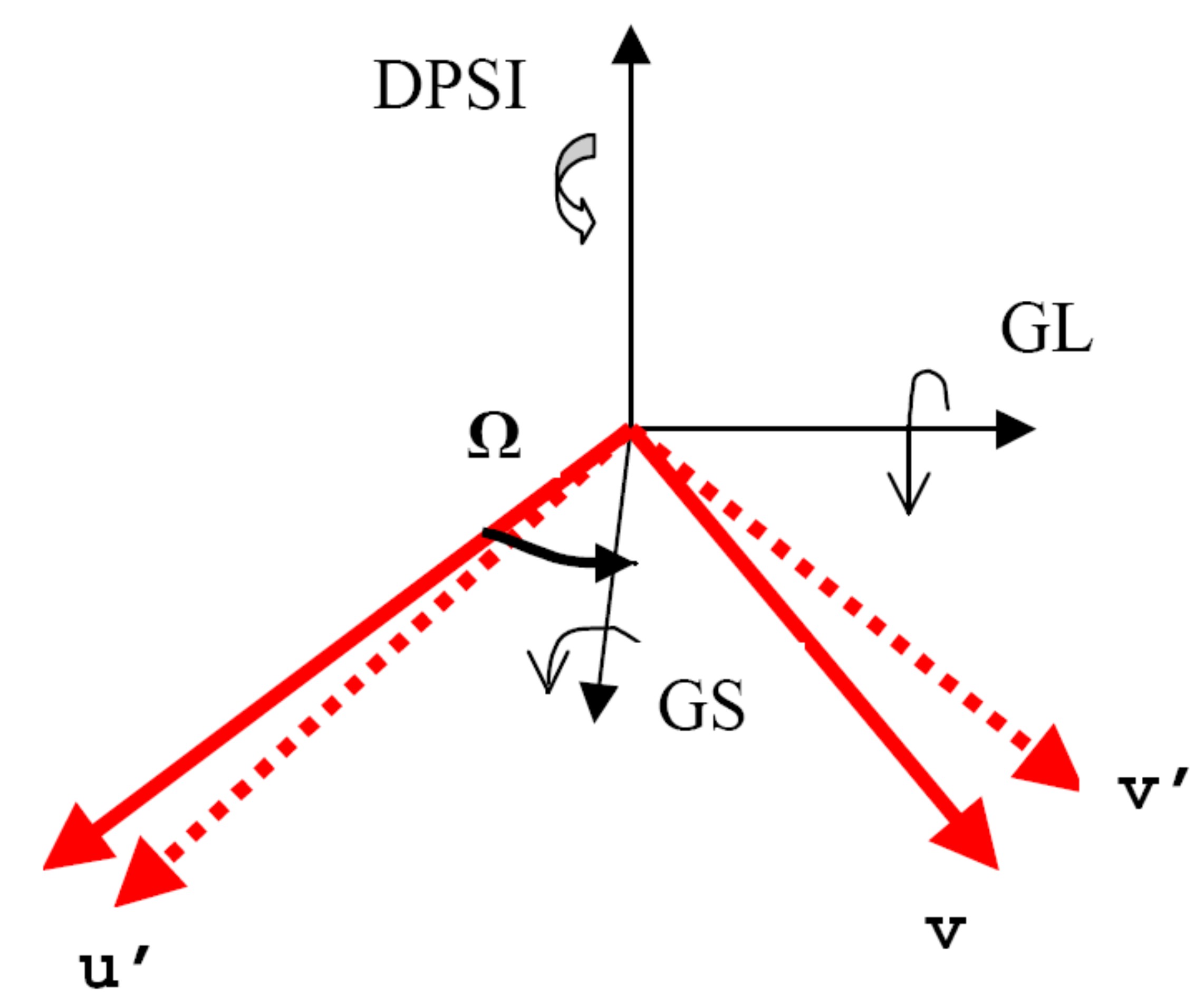
In this diagram the nominal vectors ``u`` and ``v`` are those supplied to Horace, whereas ``u``' and ``v``' are the actual vectors. gl and gs deal with misorientation about axes which lie in the spectrometer’s equatorial plane, whereas dpsi deals with misorientations about a vector perpendicular to this plane. omega is the angle by which the gs axis is rotated compared to the nominal vector ``u``.

In principle this means that you could put a single crystal with unknown orientation into the spectrometer and conduct your experiment. However this is not a good idea, because the direction about which you rotate your crystal may not be the optimum for you to get all of the data that you want to, since the detectors do not cover \(4 \\pi\) steradians.

Now we’ve told Horace all about the setup of the spectrometer we can go on to specify how our experiment was conducted and which SPE files will contribute to our dataset.

Suppose, as is the case here, we want to combine 24 SPE files, and that the angle psi was different for each one. psi is a vector, which in this case has 24 elements. We could write it out explicitly, however in our example we took data in equal steps of psi between 0 degrees and -23 degrees (1 degree steps), so we can use a Matlab trick:

nfiles=24;
psi=linspace(0,-1(nfiles-1),nfiles);

Horace needs to know the name of all 24 SPE files. To do this they are combined into a single object – a cell array, which is a Matlab data format you can read about in the Matlab help. In this case each element of the cell array is a string which specifies the location of our SPE files. We could write this out explicitly, however in this example the SPE files are numbered sequentially, so we can take another shortcut:

spe_file=cell(1,nfiles);
for i=1:length(psi)
  spe_file{i}=[indir,'MAP',num2str(11012+(2i)),'.SPE'];
end

(Note that the extension .spe;1 is not usual, normally it would be something like .spe or .SPE. Notice that it does matter whether you write the extension in lower or upper case on Windows. We have found that it does matter on, for example, Red Hat Linux).

The first line creates an empty cell array the right size to take our 24 file strings. Inside the ‘for’ loop the ith element of the cell array is a string specifying where ith SPE file. So the 5th element of the cell array spe_file is:

spe_file{5}='C:\\mprogs\\Horace\\demo\\demo_data\\MAP11022.SPE';

We are now ready to make our SQW file! This is done by a single function:

gen_sqw(spe_file,par_file,sqw_file,efix,emode,alatt,angdeg,u,v,psi,omega,dpsi,gl,gs);

If everything has worked then the Matlab command window will show text like this, which will be updated when each successive SPE file is read from the disk.

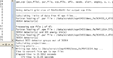
(Note that the above screenshot was created when processing a larger number of files from the same dataset as has been used for this demo. The only practical difference this makes is to the size of errorbars in 1d cuts, the time taken to process the data, and some of the on-screen printouts.)

Further through the process you should see something like this:

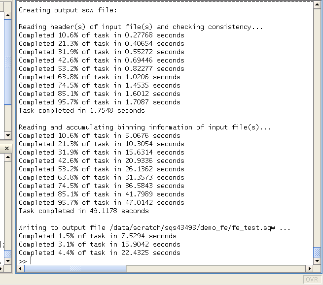
Notice that this was run on a Linux machine, hence the different style of directory name and appearance of the Matlab window.

Horace will now run for some time generating the SQW file. This can be quite a long time, and depends quite a lot on how much memory your computer has and its processor speed. It is probably best at this stage just to leave your computer to run and go for a coffee! As a rough guide 150 SPE files, each of 105MB, would be combined on a machine with 4GB of RAM (with its 3GB switch enabled) and a speed of 2.5GHz in about 2 hours.

For this demo the data files have purposely been made much smaller (by using only the low angle detector banks on MAPS, and by only including a limited number of energy bins in the SPE files). Each SPE file is about 18MB, and thus it takes about 8 minutes to process all of the data. If all is well messages will be frequently printed to the Matlab command window to let you know the status of your SQW file generation.

Data visualisation

Now that we’ve made our SQW file the next step is to see what the data look like. The first thing to do is to tell the program where the SQW file is located:

data_source='C:\\mprogs\\Horace\\demo\\ demo_fe_sqw.sqw';

which is of course the location of the SQW file we created in the previous section.

Now we have to define the projection axes for our data visualization. The projection information is contained in a structure array, which in this case we are calling proj_100. Two of the fields in this structure array are vectors. These are chosen to define the normalization (so they must be unit vectors). There are also other pieces of information that can be provided about the projection, but these will be dealt with later. So we have:

proj_100.u=[1,0,0];
proj_100.v=[0,1,0];

You can choose any (orthogonal) set of axes to make cuts and visualise your data - you are not limited to the projection axes of the crystal with respect to the spectrometer. This is one of the main advantages of using Horace to visualise your data!

Another piece of projection information that we need to know is whether the projection axes are normalised in Angstroms or reciprocal lattice units. There are 3 letters (for the 3 projection axes, the third of which is the cross product of the other two), 'r' is used for reciprocal lattice units and 'a' is used for angstroms.

proj_100.type='rrr';

Finally, we need to know if we are defining our projection axes relative to some offset. This vector has 4 components, since we could offset in energy as well as the 3 components of Q:

proj_100.uoffset=[0,0,0,0];

We now have all the information needed to make any kind of cut we like. Let’s start by making a 2D slice:

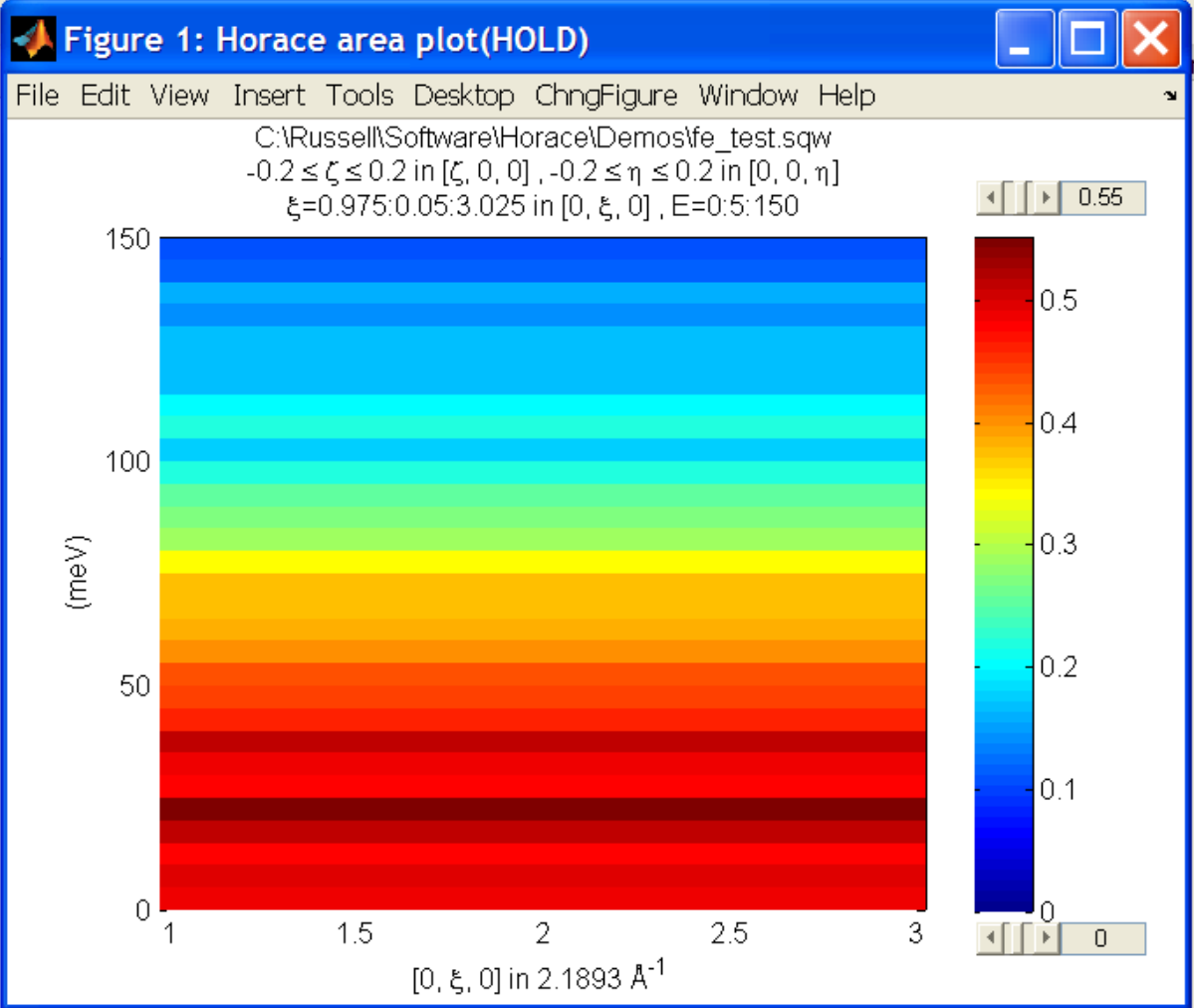
w100_2=cut_sqw (data_source,proj_100,[-0.2,0.2],0.05,[-0.2,0.2],[0,0,500]);

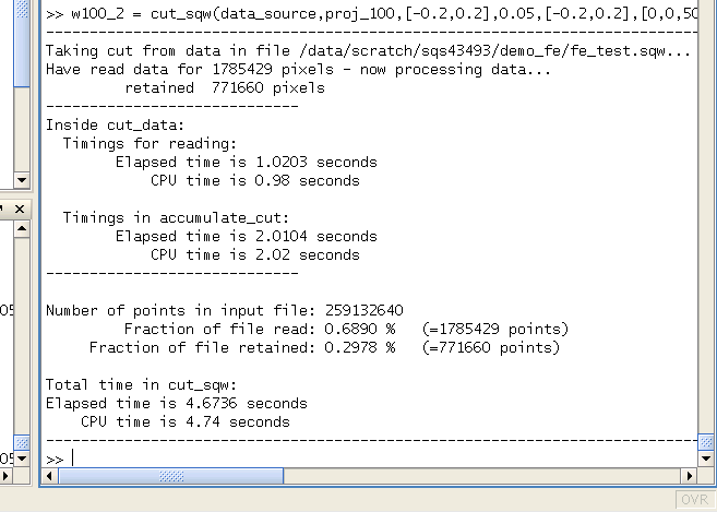
This slice has as its axes (0,1,0) and energy. The first two arguments in the function cut_sqw are where the data is on the computer, and the details of the projections. The next four arguments give either the integration range or the step size of each component of Q and energy. In this example we are integrating between -0.2 and 0.2 r.l.u. in the (1,0,0) component, and between -0.2 and 0.2 in the (0,0,1) component. The slice axes are (0,0,1) whose step size is 0.05 r.l.u., and energy whose step size is the minimum possible (this would have been specified when you Homered your data). Notice that we’ve specified the energy step size differently from the (0,0,1) step size. If a scalar is used then the whole range of data along that axis will be plotted. If a vector of the form [low,step,high] is used then only data within the range low -> high will be plotted, with step size given by step.

We don’t yet get a plot of this slice. All we’ve done here is create an ‘sqw’ object which contains the relevant information. However to plot it all we have to do is write:

plot(w100_2);

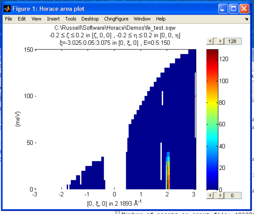
The ranges of the axes are not quite right, but we can easily change that:

lx 1 3
ly 0 150
lz 0 1

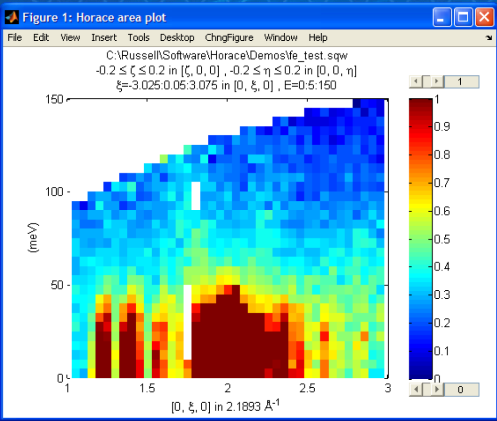
This makes the horizontal axis go from 1 to 3, the vertical axis from 0 to 150, and the colour scale go from 0 to 1.

If we wanted to make a 1D cut through the data then the syntax is exactly the same. For example:

w100_1=cut_sqw (data_source,proj_100,[-0.2,0.2],0.05,[-0.2,0.2],[60,70]);
plot(w100_1);
lx 1 3
ly 0.2 0.8

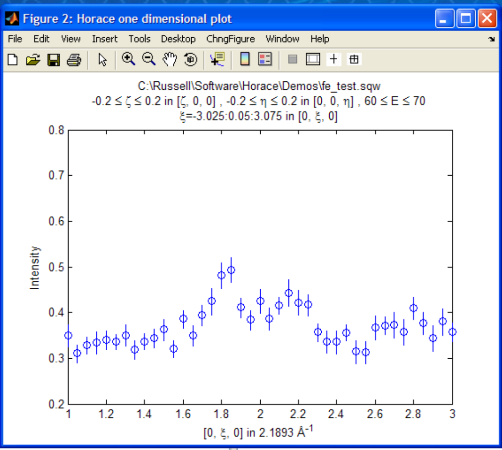
would give us a cut along the (0,k,0) axis at a constant energy of 65meV.

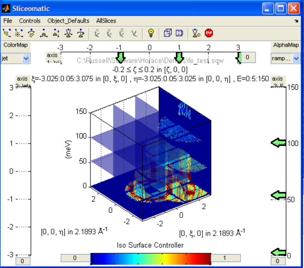
3D slices are also possible. To visualize these the ‘sliceomatic’ program is used. When the plot command is executed a GUI is launched that allows you to plot multiple slices through the data. For example you could plot the same slice with x and y axes of (1,0,0) and (0,1,0) at a range of energies.

It is possible to save your cuts / slices to be viewed again later. This can be done very simply in two ways. If you add an extra argument to the end of cut_sqw, then the cut data are sent to a file. For our 1D cut above this would be:

cut_file = 'C:\\mprogs\\Horace\\demo\\plots\\w100_1.sqw';
w100_1b=cut_sqw (data_source,proj_100,[-0.2,0.2],0.05,[-0.2,0.2],[60,70],cut_file);

Now if we want to read this in again at some later time all we need to do is type:

w100_1b = read_sqw(cut_file);
plot(w100_1b);
lx 1 3; ly 0.2 0.8

Alternatively you can store the cut data in the Matlab workspace, simply by typing:

w100_1b=cut_sqw (data_source,proj_100,[-0.2,0.2],0.05,[-0.2,0.2],[60,70]);

Note, however, that the variable w100_1b will only be stored in the Matlab workspace, so it could easily be overwritten, or lost if you quit Matlab without saving your workspace.

As we stated above, the objects that you created using the cut_sqw and cut commands are all of the type ‘sqw’. These are the generic objects dealt with by Horace and can represent data that is 0 to 4- dimensional. The sqw objects contain information about the contributing pixels to the cut, which in principle allow things like resolution corrections to be done when you analyse your data. However, in some instances you may not wish to retain this information, for example if you are dealing with lots of large 4-dimensional objects and are worried about running out of memory, or if you do not intend to use the pixel information. If this is the case there are two things you can do, depending on whether you are cutting data from a file or from an object in memory. If cutting data from a file and you do not wish to retain pixel information then the syntax is

w100_2_nopixels=cut_sqw (data_source,proj_100,[-0.2,0.2],0.05,[-0.2,0.2],[0,0,500],'-nopix');

If cutting data from an sqw object in memory then the syntax is

w100_1d=cut(w100_2,0.05,[60,70],'-nopix');

where w100_2 is the 2-dimensional sqw object created earlier.

If you make a cut to create an object that is 2-dimensional, but with no pixel information, then it becomes a new type of Horace object – in this case a ‘d2d’. If the cut creates a 1-d object then it is known as a ‘d1d’, and so on. Most operations that apply to sqw objects also apply to dnd objects, albeit appropriately modified, e.g. the command plot applies to both kinds of data. The most notable difference applies to simulation and fitting of data.

Basic data manipulation

Horace allows you to manipulate your data in many different ways. The number of manipulation functions supplied with the standard download is quite small, however it is relatively easy to write your own bespoke functions – the syntax can be worked out by looking at the existing functions.

It is important to realise that there are essentially 3 different kinds of function, each with a slightly different syntax. The first set of functions, which will be described first below, are ones which take an existing data set and manipulate it in some way before returning the manipulated dataset. An example of this would be dividing the entire dataset by the Bose factor.

The second kind of function is a general function which takes a number of input vectors, corresponding to the axes of the desired output object and performs a mathematical operation on them to give an n-dimensional output. An example of this would be a function called something like gauss_2d which takes two vectors that specify a grid in (Q,E)-space and some parameter, and returns a 2D grid with an intensity modeled by a Gaussian.

The final kind of function is a ‘proper’ model of S(Q,E), i.e. one which takes all of the values of Q and E for a particular dataset and calculates a dispersion relation, say, which is then plugged into a simple harmonic oscillator response function.

With the above caveats in mind, let’s demonstrate two different kinds of data manipulation of the first type discussed above. In the first we will simulate the background for a 2D slice by looking at the signal at high |Q| in a 1D cut and then replicating it into 2D and subtracting from the real data. We’ll then demonstrate correcting the data for the Bose-Einstein thermal population factor.

First create a new 2D slice and save to file:

cut_file = 'C:\\mprogs\\Horace\\demo\\ w110.sqw';
cut_sqw (data_source, proj_110, [-0.2,0.2], [1,0.05,5], [-0.2,0.2], [0,0,150], cut_file);
w110 = read_sqw(cut_file);

Now make a 1D cut out of this slice along the energy axis, with the integration range along (0,1,0) of 4.8 to 5:

wbackcut = cut(w110,1,[4.8,5]);

Next make a new 2D slice by replicating the cut along one of the integration axes:

wback = replicate(wbackcut,w110);
plot(wback);

This is a 2D slice that is over the same range as w110. We now subtract this from the real data:

wdiff = w110-wback;
plot(wdiff);

Simulations

It is not only possible to plot and manipulate data, it is also possible to simulate an entire dataset, or parts of a dataset. We will illustrate this option using two examples, one that gives a quartet of Gaussian profile peaks, and another that simulates the intensity from a Heisenberg ferromagnet.

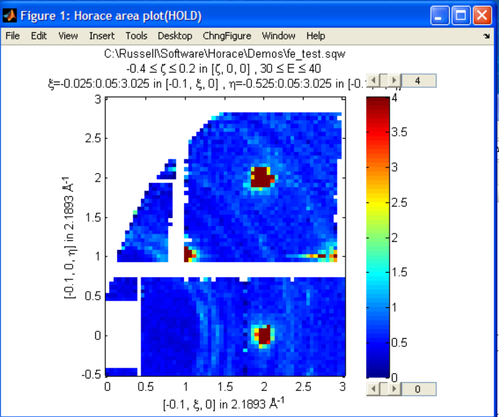
It is often the case that you do not have a full model of S(Q,E), but rather you just want to determine how a particular peak changes with, for example, temperature or neutron energy transfer. An example would be to monitor the positions and intensities of a quartet peaks. We can generate a slice from our demo data by typing:

w_template=cut_sqw(data_source,proj_100,[-0.4,0.2],[0,0.05,3],[-0.5,0.05,3],[30,40]);

This should give a plot that looks like this:

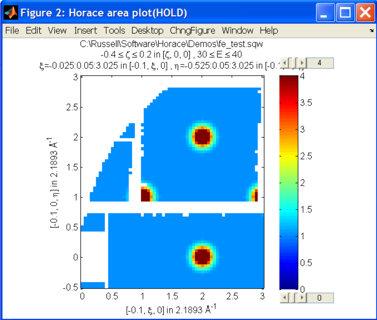
We will now simulate this using the demonstration function demo_4gauss. This is a specially written function which works only for 2D datasets (slices) where both axes are momentum. Read through the code in

C:\\mprogs\\Horace\\functions\\demo_4gauss.m

to see if you can understand how the function works… It is a far from simple task to write a function that is completely general for any dimensionality of dataset, so you typically write functions such as this that work only for a particular dimensionality. It is important, therefore, for your own book-keeping, that you give the functions sensible names that reflect both what they do and what sort of dataset they apply to.

Now let’s run the function. Instead of using user_func we will use func_eval. The syntax for functions called by this routine is slightly different:

w_sim= func_eval (w_template,@demo_4gauss,[6 1 1 0.1 1.25 6 1]);

The arguments in the square parentheses are the function inputs, and in this case they correspond respectively to amplitude, satellite position x-coordinate, satellite y-coordinate, central position x-coordinate, central y-coordinate, and background. In general the input to a function called by func_eval can take any form (e.g. a cell array, a structure array, a string, etc.), although if you wish to pass anything other than a vector of parameters, such as that shown above, then it must be packed into a cell array.

Notice that the syntax of the input arguments is somewhat different for func_eval compared to user_func, since with the former we input the parameters as a vector, rather than as separate arguments. The form of the function itself is also different, since it takes some arrays of parameters and calculates an intensity at those points, rather than taking an existing intensity array and modifying it.

func_eval works for both sqw and dnd objects with almost the same syntax. For sqw objects pixel information is simulated according to the intensity calculated for the data grid, whereas for dnd objects this is not required. It is also possible to simulate a dnd from a template sqw object by using an additional keyword argument of the form

dnd_sim= func_eval (w_template,@demo_4gauss,[6 1 1 0.1 1.25 6 1],'all');

Furthermore one can use the same keyword argument on a template dnd object so that intensity is simulated over the entire data range, rather than just at the points where there are data in the template object.

There is another way of performing a simulation, using a different method and a simulation function with a slightly different input structure. In this case you are fitting a full model of S(Q,E), so the function we will demonstrate here is a model appropriate for spin excitations of a 3D Heisenberg ferromagnet. The function is called FM_spinwaves_2dSlice_sqw, and it takes as its inputs arrays (or scalars) for all 3 components of Q plus energy, as well as the other function parameters (exchange constant etc.). The format of the inputs for this function are thus different from those of demo_4gauss - to see the differences it is probably easiest to examine the code for the two functions side-by-side.

w_sim= sqw_eval (w_template,@FM_spinwaves_2dSlice_sqw,[300 0 2 10 2]);

In general it is better to use func_eval for simple functions such as Gaussians and so on, and sqw for “proper” models of the scattering. The different syntax makes it easier to keep track of what kind of model for the scattering is being employed. As before, the keyword ‘all’ can be added to the arguments of this function, however in this case it is ignored if the object w_template is an sqw object. If w_template is a dnd object then as for func_eval the keyword ‘all’ ensures that data are simulated over the entire data range. As with func_eval, the parameters passed to the function can either take the form of a vector of numerical parameters, or a cell array comprising any other form of input.

Fitting

You can also use Horace to fit your data. It can take quite a long time for the fit to converge, so it is therefore a good idea to provide a good initial guess of the fit parameters. You can work these out simulating and then comparing the result to the data by eye.

For an introduction and overview of how to use the following fitting functions, please read Fitting data. For comprehensive help, please use the Matlab documentation for the various fitting functions that can be obtained by using the doc command, for example doc d1d/multifit (for fitting function like Gaussians to d1d objects) or doc sqw/multifit_sqw (fitting models for S(Q,w) to sqw objects).