Resolution Convolution

Horace includes support for calculating the effect of instrument resolution on a model simulation and fitting.

Theory Background

Horace is designed for time-of-flight (ToF) inelastic neutron data from multi-detector spectrometers. The detectors measure the angle at which a neutron is scattered from the sample, and the neutron’s time of arrival, which is used to determine its speed. The data is binned in ToF and this is converted into a nominal energy transfer \(\omega_0\). The angular position of the detector together with the energy information gives a nominal momentum transfer from the sample \(\mathbf{Q}_0\).

The neutron beam, however, is neither perfectly collimated nor perfectly monochromatic. As such, there is a spread of neutron velocities and angles in a physical instrument which results in an instrumental resolution broadening. This can be described by a resolution function \(R(\mathbf{Q}-\mathbf{Q}_0, \omega - \omega_0) = R(\delta\mathbf{Q}, \delta\omega)\) where \(\mathbf{Q}\) is the true momentum transfer and \(\omega\) is the true energy transfer for a given detected neutron.

The measured neutron counts at a detector-energy element whose centre is at \((\mathbf{Q}_0, \omega_0)\) is thus:

\[I(\mathbf{Q}_0, \omega_0) = \int R(\delta\mathbf{Q}, \delta\omega) S(\mathbf{Q}, \omega) d\mathbf{Q} d\omega\]

Horace calculates this resolution broadening using a Monte Carlo method, by sampling points within the distribution \(R(\delta\mathbf{Q}, \delta\omega)\), and averaging over them. That is, for each detector-energy element it determines \(N\) deviations \((\delta\mathbf{Q}_i, \delta\omega_i)\) drawn from \(R\) and evaluates the model function \(S\) at these new coordinates, computing the resolution-convolved intensity as:

\[I(\mathbf{Q}_0, \omega_0) = \frac{1}{N} \sum_{i=1}^{N} S(\mathbf{Q}_0+\delta\mathbf{Q}_i, \omega_0 + \delta\omega_i)\]

By default \(N=10\) is used because often there are many detector-energy elements (pixel in Horace syntax) which contribute to a single bin (histogram), so there is already some broadening included. This means, though, that resolution calculations takes \(N\) times longer than non-resolution convolved calculations. The value of \(N\) is set using the set_mc_points method of the tobyfit class.

The distribution \(R(\delta\mathbf{Q}, \delta\omega)\) is computed analytically in Horace, except for a “work-around” for modern neutron guides described below. Horace considers 11 variables which contribute to the resolution broadening, ranked in order of importance:

• \(t_m\) - the time deviation at the moderator (time at which a neutron is emitted which is not \(t=0\))

• \(y_a\), \(z_a\) (or \(\gamma_y\), \(\gamma_z\)) - The coordinates of the neutron at the aperture (this is the effective angular view the spectrometer has of the moderator). Originally, the theory described here 1 applied only to instruments without neutron guides, so it was assumed that the neutron beam’s angular divergences \((\gamma_y, \gamma_z)\) can be determined simply by the size of the aperture / viewport onto the moderator. (Horace uses a laboratory coordinate system where \(x\) is the beam direction, \(y\) is horizontal perpendicular to the beam and \(z\) is vertical). Modern neutron guides are accommodated in this formulism by pre-calculating the (incident energy dependent) divergences using a neutron ray-tracing code (McStas in this case) and using look-up tables in the code.

• \(t_{ch}\) - the time deviation at the chopper (e.g. the chopper opening time)

• \(x_s\), \(y_s\), \(z_s\) - the neutron coordinate where it scatters at the sample.

• \(x_d\), \(y_d\), \(z_d\), \(t_d\) - the neutron coordinate at the detector

The last two sets (neutron coordinates at the sample and detector) represent the geometrical uncertainty in the neutron’s angle and time of arrival due to the finite sizes of the sample and detector. In practice, they contribute relatively little to the resolution broadening but may be important for large samples.

The 11 variables above are sampled to produce an 11-dimensional vector \(\mathbf{Y} = (t_m, y_a, z_a, t_{ch}, x_s, y_s, z_s, x_d, y_d, z_d, t_d)\) in the laboratory frame. This is mapped to the sample frame by a linear transformation:

\[(\delta\mathbf{Q}, \delta\omega) = \mathbf{T} \mathbf{B} \mathbf{Y}\]

where the \(\mathbf{T}\) and \(\mathbf{B}\) matrices are given in Appendix A of Ref 1, in equation A66 and Table A1 respectively 2.

The Tobyfit class

For historical reasons, the subclass of multifit which handles resolution convolution is called tobyfit. The intent is make the simulation of a resolution-convoluted model almost the same as without resolution convolution.

For example, given a cut w1 and a model function @model_fun we can set up a fitting problem in the ordinary case with:

kk = multifit_sqw(w1);
kk = kk.set_fun(@model_fun, initial_parameters)
kk.fit()

To include resolution convolution we have to specify some additional information on the sample and instrument (spectrometer) configuration, for example:

w1 = set_sample(w1, IX_sample([0,0,1],[0,1,0],'cuboid',[0.01,0.05,0.01]));
w1 = set_instrument(w1, maps_instrument(70, 300, 'S'));
kk = tobyfit(w1);
kk = kk.set_fun(@model_fun, initial_parameters)
kk.fit()

We can see that aside from two additional lines to append sample and instrument information to the cut w1 the fitting syntax is exactly the same.

The IX_sample class has the following signature:

sample = IX_sample (xgeom, ygeom, shape, ps, eta, temperature)

• xgeom and ygeom are vectors in reciprocal lattice units defining the directions of the sample’s \(x\) and \(y\) axes for definition of the shape parameters ps.

• shape is a string defining what shape the sample has. Only point and cuboid are accepted at present.

• ps is a vector of shape parameters. For the cuboid shape it is a 3-element vector of the dimensions in metres of the sample in the \(x\), \(y\), and \(z\), where these directions are defined w.r.t. the crystal orientation by the xgeom and ygeom arguments.

• eta (optional) is the crystal mosaic spread FWHM in degrees (isotropic mosaicity), or an IX_mosaic object for anisotropic mosaicity - type doc IX_mosaic/IX_mosaic for more information.

• temperature (optional) is the sample temperature in Kelvin.

For the instrument information, there are 3 helper functions covering the ISIS direct geometry spectrometers which can measure single crystals:

• merlin_instrument(ei, hz, chopper)

  • ei is the incident energy in meV

  • hz is the chopper frequency in Hz

  • chopper is the chopper rotor package type, a string either 'sloppy', 's' or 'g'.

• maps_instrument(ei, hz, chopper, '-version', inst_ver)

  • ei and hz as above.

  • chopper can be either 's' or 'a'.

  • inst_ver can be:

    • 1 - MAPS from 2000 to 2016 (without a neutron guide)

    • 2 - MAPS since 2017 after the guide upgrade.

• let_instrument(ei, hz5, hz3, slot_mm, mode, '-version', inst_ver)

  • ei is the incident energy of this rep (not the focussed Ei)

  • hz5 is the frequency of Chopper 5 in Hz

  • hz3 is the frequency of Chopper 3 in Hz

  • slot_mm is the full width of Chopper 5 in mm. Depending on instrument version it is:

    • inst_ver=1 - slot_mm must be 10 mm.

    • inst_ver=2 - slot_mm can be one of 15, 20, 31 mm, corresponding to “High resolution”, “Intermediate” and “High Flux” modes

  • mode - running mode of Chopper 1 (pulse shaping) chopper. One of:

    • mode=1 - “High resolution” mode with hz1 = hz5 / 2

    • mode=2 - “High flux” mode with hz1 = hz3 / 2

  • inst_ver can be:

    • 1 - LET until autumn 2016 (with the original double funnel snout at Chopper 5).

    • 2 - LET since autumn 2016 (with a single focusing final guide section).

In addition to the above parameters all instruments also take a optional 'mod_value' argument specifying the type of moderator pulse model to use. At present, only two options are available:

• 'empirical' - based on the Ikeda-Carpenter distribution of Ref 3 (default).

• 'base2016' - a look-up table from ray-tracing simulations of ISIS moderators in 2016.

For the empirical model, there is also an option to refine the parameters which define the model as described below.

Once the sample and instrument setup information is configured on a workspace, a fitting or modelling problem can be defined using the tobyfit class in place of multifit_sqw. The exact same syntax as multifit for defining fixed and free parameters and background can then be used in tobyfit.

In addition to standard multifit methods (set_fun, set_free etc), there are some additional methods specifically for the resolution convolution:

• kk = kk.set_mc_points(n) - sets the number of Monte Carlo points per pixel (default \(N=10\)).

• kk = kk.set_mc_contributions(contrib1, contrib2, ...) - sets which instrument component contributes to the Monte Carlo sum. contrib1 etc are strings, and can also be 'all' (default) or 'none'. The contributions depend on the instrument and can be listed with kk.mc_contributions. In addition, you can specify to include all contribution except certain ones with 'no<contrib>'. E.g. kk = kk.set_mc_contributions('nosample') will include all contribution except for the 'sample' contribution.

• kk = kk.set_refine_moderator(true) - tells Horace to try to refine the moderator pulse width model concurrently with running a fit. That is, the moderator model parameters will be added to the list of model parameters and will be fitted at the same time as the user model parameters when kk.fit() is called.

The last option only has effect if an empirical moderator model is chosen (which is the default for all instruments). In addition to the syntax above, you can also use an alternative syntax which specifies initial values for the moderator model and if any of those parameters should be fixed:

kk = kk.set_refine_moderator(model_name, initial_pars, vary);

Only 'ikcarp' is valid as a model_name at present. This model takes three parameters: initial_pars = [tau_f, tau_s, R] where tau_f is the fast decay time in microseconds (\(\tau_f = 1/\alpha\) compared to the Ikeda-Carpenter paper 3), tau_s is the slow decay time in microseconds (\(\tau_s = 1/\beta\) in Ikeda-Carpenter’s notation), and R is the weight of the storage term.

Note

By default, Horace sets tau_f = 70/sqrt(Ei), tau_s = 0 and R = 0. That is, it uses a simple \(\chi^2\) distribution with only the fast decay term.

vary is a 3-element logical vector of which parameters to vary.

For example, to fit an empirical moderator model varying only the fast decay term use:

tauf=5; taus=25; R=0.3; vary = [1, 0, 0];
kk = kk.set_refine_moderator ('ikcarp', [tauf, taus, R], vary)

A worked example

The following script will make a cut from a data file, set up a fitting problem with resolution convolution, run a simulation and plot it. It uses data on bcc-Iron, which can be downloaded here. The model function is an analytic spin-wave model, defined by a dispersion relation:

\[E_0(q_h, q_k, q_l, E) = \Delta + 8 J \left(1 - \cos(\pi q_h) \cos(\pi q_k) \cos(\pi q_l) \right)\]

convolved with a Gaussian line shape. The next section has a better model with a harmonic-oscillator line shape which fits the data better. We have chosen the simpler model here so it can fit into a Matlab anonymous function.

% Make cut
proj = projaxes([1,1,0], [-1,1,0], 'type', 'rrr');
w1 = cut_sqw('fe_cut.sqw', proj, 0.05, [-1.05,-0.95], [-0.1,0.1], [80, 100])

% Define the instrument and sample information on the cut
xdir = [1,0,0]; ydir = [0,1,0]; ei = 401; freq = 600; chop_type = 's';
w1 = set_sample(w1, IX_sample(xdir, ydir, 'cuboid', [0.03,0.03,0.03]));
w1 = set_instrument(w1, maps_instrument(ei, freq, chop_type));

% Define a fitting / model function
% (spin waves in bcc-Iron with Gaussian peak shape and magnetic form factor).
ff_fun = MagneticIons('Fe0').getFF_calculator(w1);
E0 = @(h,k,l,e,js,d) d + (8*js) .* (1 - cos(pi * h) .* cos(pi * k) .* cos(pi * l));
fe_sqw_ff = @(h,k,l,e,p) (p(4)/p(3)) * transpose(ff_fun(h,k,l,e,[])) ...
    .* exp(-((e - E0(h,k,l,e,p(1),p(2))) ./ p(3)) .^2)

% Set initial parameters
J = 35; d = 0; sigma = 25; amp = 150;

% Set up tobyfit object
tf = tobyfit(w1);
tf = tf.set_fun(fe_sqw_ff);
tf = tf.set_pin([J d sigma amp]);
tf = tf.set_bfun(@linear_bg);
tf = tf.set_bpin([0.2 0]);

% Run the simulation and plot
wsim = tf.simulate()
acolor('k'); plot(w1); acolor('r'); pl(wsim)

% Run it again without resolution convolution
kk = multifit_sqw(w1);
% We can also set input pars when we define the model function
kk = kk.set_fun(fe_sqw_ff, [J d sigma amp]);
kk = kk.set_bfun(@linear_bg, [0.2 0]);
wnores = kk.simulate()
acolor('k'); pl(wnores);

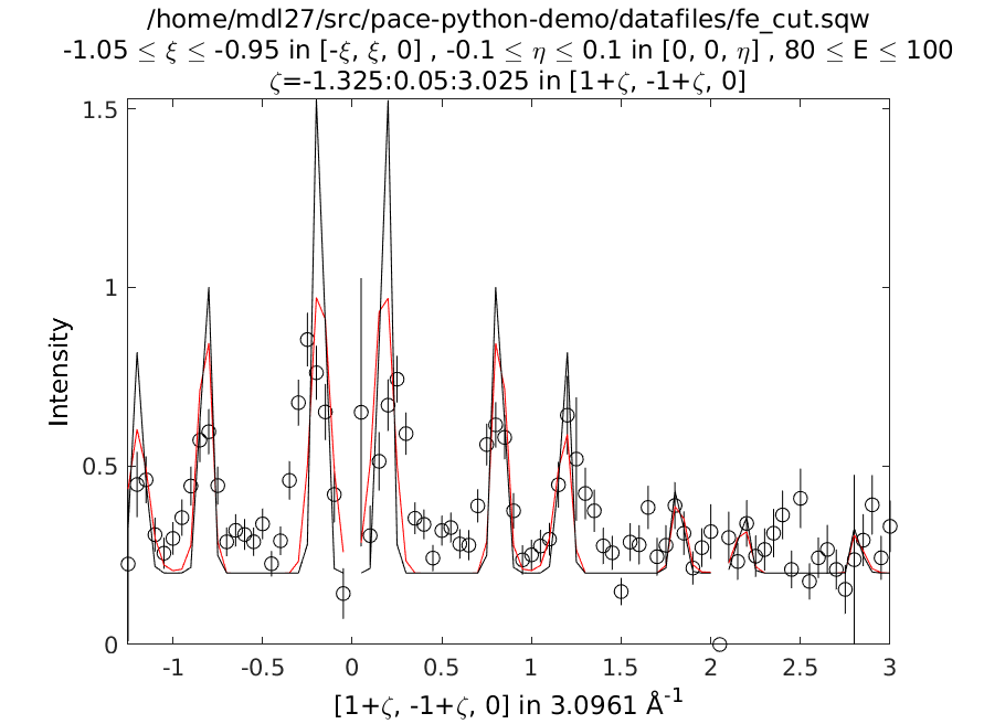
A constant energy cut along \([110]\) centred at 90 meV of the Iron dataset with a model calculation including instrument resolution (red) and without (black lines).

Plotting resolution ellipsoids

Finally, Horace can also plot a resolution ellipsoid over a 2D plot (only 2D color plots are supported at present):

proj = projaxes([1,1,0], [-1,1,0], 'type', 'rrr');
w1 = cut_sqw('fe_cut.sqw', proj, 0.05, [-1.1,-0.9], [-0.1, 0.1], [50,5,120]);
xdir = [1,0,0]; ydir = [0,1,0]; ei = 401; freq = 600; chop_type = 's';
w1 = set_sample(w1, IX_sample(xdir, ydir, 'cuboid', [0.03,0.03,0.03]));
w1 = set_instrument(w1, maps_instrument(ei, freq, chop_type));
resolution_plot(w1)

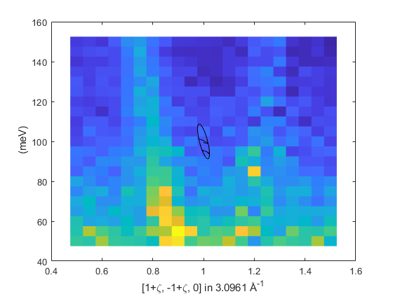
The above command plots a resolution ellipsoid at the centre of the cut. To plot it at a specified (2D) projected coordinate, use resolution_plot(w1, proj_coord) where proj_coord is a 2-element vector of the coordinate in the projection of the cut, or an \(N \times 2\) array of such coordinates.

The function can also optionally return the covariance matrices at the desired point:

[cov_proj, cov_spec, cov_hkle] = resolution_plot(w1, proj_coord)

where each return value is a \(4 \times 4 \times N\) array of covariance matrices in the projection axes coordinate (cov_proj), the spectrometer Cartesian axes (cov_spec, with \(x\) along the beam, \(z\) vertical and \(y\) horizontal perpendicular to the beam direction), or the crystal coordinates (cov_hkle).

References

1(1,2)

T. G. Perring, High Energy Magnetic Excitations in Hexagonal Cobalt, Ph.D. Thesis, University of Cambridge, 1991. Also published as RAL Technical Report RALT-028-94

2

The matrix elements may also be obtained from the Horace source code here. Note that the \(T\) matrix is called qk_mat.

3(1,2)

S. Ikeda and J. M. Carpenter, Nucl. Inst. and Meth. in Phys. Res. A239, pp536 (1985)