Interfacing with other programs

Horace is designed to be able to call other programs to calculate models for simulating and fitting data.

This document describes two interfaces with other PACE projects:

• Euphonic

• SpinW

as well as a generic way of interfacing with modelling codes you may want to use with Horace.

We also note that the Brille library for \(q\)-space interpolation is also a PACE project and is used internally by Euphonic and SpinW to speed up calculations. Documentation for how to accomplish may be found in the relevant Euphonic and SpinW documentation.

Recap on evaluating functions on a Horace workspace

As described in the Simulation section, Horace takes two types of model functions:

• User model functions which operate on the \((x,y,z,e)\) coordinates of a particular cut, evaluated using func_eval and similar functions.

• User model functions which operate on the \((\mathbf{Q}, \omega)\) coordinates, evaluated using sqw_eval and similar functions.

In the first case, for example, if the user makes a 1D cut along the \(\mathbf{Q}=(1,1,0)\) direction, and calls func_eval on this cut, a single vector of the values of \(\sqrt{Q_h^2 + Q_k^2}\) is passed to the user model function. On the other hand, if she calls sqw_eval on this cut, 4 vectors, namely \((Q_h, Q_k, Q_l, E)\), are passed to the user model function. Generally, “simple” functions such as linear backgrounds or peak functions (Gaussians, Lorentzians, etc), are used with func_eval whilst more complex models use sqw_eval. In particular the interface with external modelling codes described here exclusively use the second type.

Energy convolution

The sqw_eval function expects the user model function to return a single vector \(S(Q_h, Q_k, Q_l, E)\) of neutron intensity evaluated at the 4 reciprocal space coordinates. However, in many cases calculations instead return pairs of values \((E, I)\) of mode energy \(E\) and intensity \(I\) for a particular \(\mathbf{Q}=(Q_h, Q_k, Q_l)\) point. This is the case for phonon calculations, where at each \(\mathbf{Q}\) point a dynamical matrix is constructed whose eigenvalues are the mode energies squared and whose eigenvectors can be used to calculate the dynamical structure factor which is proportional to \(I\).

In these cases, an energy convolution has to be performed to obtain \(S(Q_h, Q_k, Q_l, E)\). This can be done with the disp2sqw_eval function. This function passes the needed \((Q_h, Q_k, Q_l)\) to the model function and performs an energy convolution using either:

• A fixed width peak function (Gaussian by default)

• Energy-variable width peak function, where the peak width varies with energy transfer

• A custom user defined shape function (for \(\mathbf{Q}\) and \(E\) dependent peak shapes).

Note that this energy convolution is required for all model functions which yields pairs (energy \(E\), intensity \(I\)) from an input set of \(\mathbf{Q}=(Q_h, Q_k, Q_l)\) points. For calculations which take into account the instrument resolution function, this energy convolution can be considered the “intrinsic” (lifetime) energy broadening of the excitation.

Euphonic example

Installing Euphonic

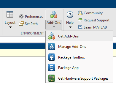
Euphonic is a Python package to calculate phonon inelastic neutron scattering (INS) intensities from force constants determined from ab initio calculations. To use it with Horace, you should first download the Horace-Euphonic-Interface which is available as a Matlab toolbox add-on. This can be installed within Matlab by clicking on the “Home” tab in the control ribbon, then clicking “Add-Ons” and “Get Add-Ons”:

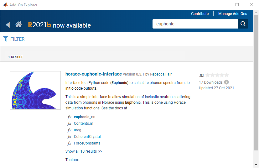
Type euphonic in the search bar, and click on the horace-euphonic-interface package.

Then click “Add” in the next window (you may have to log into your Mathworks account).

If you prefer, you can download the Horace-Euphonic-Interface toolbox directly from here (download the latest mltbx file). Then run:

matlab.addons.toolbox.installToolbox('/path/to/mltbx_file')

Because Euphonic is a Python program, you need to have Python setup on your system, and to tell Matlab about this. Please see here for more detailed information.

If you haven’t installed the Euphonic Python package then you can do this within Horace using:

euphonic.install_python_modules()

This may not work for all Python distributions, in which case you should install Euphonic manually. Euphonic can be installed with pip install euphonic in the Python command line, but there are also other ways of installing Euphonic, which are detailed in the Euphonic installation instructions.

On the IDAaaS system, you can access the pre-installed Euphonic Python environment using:

pyenv('Version', '/usr/local/virtualenvs/euphonicenv/bin/python3');
py.sys.setdlopenflags(int32(10));

Note that this should be done at the start of a Matlab session. If a different Python interpreter has already been started you will need to restart Matlab, otherwise the above command will give an error.

To test that Euphonic has been installed correctly, run:

help(euphonic.ForceConstants)

Which will give you the (Python) help text on the ForceConstants class. If Euphonic was not installed correctly, this command will give an error.

Running a Euphonic calculation with Horace

To perform a phonon INS calculation Euphonic requires the force constants from an ab initio calculation. Euphonic can read this information from either a CASTEP .castep_bin file using the from_castep() method, or a Phonopy output folder containing a phonopy.yaml file using the from_phonopy() method.

In addition to reading in the force constants, we must also set certain parameters for the INS calculation. To do this we create a CoherentCrystal object from the ForceConstants data we read in. This CoherentCrystal has a method (function), horace_disp() which can be passed to the Horace disp2sqw_eval function.

The following code reads the force constants from a CASTEP file, sets up the CoherentCrystal object and then evaluate the phonon model on an experimental cut:

% Read force constants
fc = euphonic.ForceConstants.from_castep('quartz.castep_bin')

% Set up model
coh_model = euphonic.CoherentCrystal(...
   fc, ...
   'conversion_mat', [1 0 0; 0 1 0; 0 0 -1], ...
   'debye_waller_grid', [6 6 6], ...
   'temperature', 100, ...
   'asr', 'reciprocal', ...
   'use_c', true);

% Read in experimental cut
cut = cut_sqw('quartz_cut.sqw', [-3.02, -2.98], [5, 0.5, 38])

% Simulate
scale_factor = 200;
effective_fwhm = 1;
cut_sim = disp2sqw_eval(...
   cut, @coh_model.horace_disp, {scale_factor}, effective_fwhm);

% Plot
plot(cut_sim);

Note

The data files quartz.castep_bin and quartz_cut.sqw are available for download here

• The conversion_mat parameter denotes a \(3 \times 3\) matrix to transform from the \(q\)-points in Horace to that used by the phonon model (i.e. that used in the ab initio calculation). This is needed if, for example, a primitive unit cell is used in the ab initio calculation but the Horace data is defined using a conventional unit cell. By default it is set to the identity matrix.

• The debye_waller_grid parameter is the size of the (Monhkhorst-Pack) \(q\)-space grid to use for the Brillouin zone integration needed to calculate the Debye-Waller factor. Higher values will yield a more accurate calculation but the \(6 \times 6 \times 6\) is sufficient in most cases.

• The temperature is in Kelvin.

• The asr parameter specifies whether and how the acoustic sum rule (ASR) correction should be applied:

  • reciprocal applies the ASR correction to the dynamical matrix at every \(q\)-point (recommended).

  • realspace applies the ASR correction is applied to the force constant matrix in real space. This method is known to fail for polar systems.

  If this parameter is not specified, the ASR correction is not applied. This means that the phonon modes are not enforced to have zero energy at the \(\Gamma\) point, and the dispersion close to \(\Gamma\) may not be linear. It’s generally best to specify it in the reciprocal mode.

• The use_c parameter specifies whether to use the compiled C extension module for faster calculation or not.

For further information and other options, type help(euphonic.CoherentCrystal) in the Matlab command window.

Fitting data with Euphonic and Horace

Fitting in Horace uses the multifit application. After running the above code, a fit can be performed using:

kk = multifit_sqw(cut);
kk = kk.set_fun(@disp2sqw, {@coh_model.horace_disp, {scale_factor}, effective_fwhm});
[fitted_cut, fit_pars] = kk.fit();

Because Euphonic uses ab initio data, the only “fittable” parameters are scale factors. By default, only the intensity scale factor is fitted to the data. If you wish, you can also fit an overall energy scale factor, by giving an extra value in the input cell:

kk = kk.set_fun(@disp2sqw, {@coh_model.horace_disp, {[scale_factor energy_scale]}, ...
                effective_fwhm});

This syntax is also ideally suited to simulating a phonon model with instrument resolution convolution as described in the last section:

% Defines the sample geometry.
is_crystal = true;
xgeom = [0,0,1]; ygeom = [0,1,0];
shape = 'cuboid'; shape_pars = [0.01,0.05,0.01];

% Need to set the sample information inside the cut.
cut = set_sample(cut, IX_sample(is_crystal, xgeom, ygeom, shape, shape_pars));

% Do the same for the instrument information
ei = 40; freq = 400; chopper = 'g';
cut = set_instrument(cut, merlin_instrument(ei, freq, chopper));

scalefac = 1e12;
intrinsic_fwhm = 0.1;
tt = 5;  % temperature in K

kk = tobyfit(cut);
kk = kk.set_fun(@disp2sqw, {@coh_model.horace_disp, {scale_factor}, intrinsic_fwhm});
sim = kk.simulate('fore');

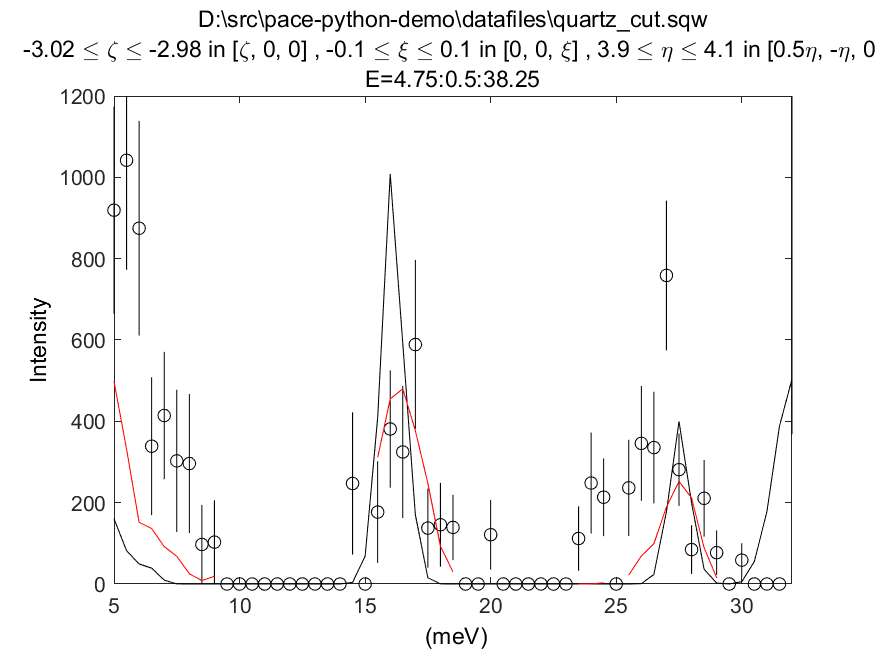
% Plots the data (black points), non-resolution convoluted simulation (black lines)
% and resolution-convoluted simulation (red lines)
acolor black; plot(cut); pl(cut_sim); acolor red; pl(sim)

In this case, the energy width parameter is an intrinsic (lifetime) width instead of an effective width which includes contribution from both instrument resolution as well as lifetime broadening.

SpinW example

Installing SpinW

SpinW is a Matlab program to calculate magnetic inelastic neutron spectra using linear spin wave theory (LSWT). It is available as an “Add-On”, and can be installed similarly to the Horace-Euphonic-Interface above (search for spinw instead of euphonic!).

Alternatively, you can download the zipped release distribution and extract it to a folder and then add that folder to the Matlab path using addpath(genpath('/path/to/spinw')).

Running a SpinW calculation with Horace

Similarly to the Euphonic horace_disp() method, the spinw class has a horace_sqw method which is used as a gateway between SpinW and Horace.

horace_sqw acts as a wrapper around the spinwave and sw_neutron functions which carry out the actual spin wave INS calculations in SpinW. In addition, it also carries out the energy convolution described in the Energy convolution section above.

A user should set up a SpinW model and then pass a handle (indicated by the @ operator) to the horace_sqw method to sqw_eval or directly to a multifit object, for example:

% Set up a simple triangular lattice antiferromagnet model
J = 1.2; K = 0.2; fwhm = 0.75; scalefactor = 1;
tri = sw_model('triAF', J);
tri.addmatrix('label', 'K', 'value', diag([0 0 K])); tri.addaniso('K');

% Make a cut of some data
ws = cut_sqw(sqw_file, [0.05], [-0.1, 0.1], [-0.1, 0.1], [0.5]);

% Set up the fitting problem
kk = multifit_sqw(ws);
kk = kk.set_fun(@tri.horace_sqw);
kk = kk.set_pin({[J K fwhm scalefactor], 'mat', {'J_1', 'K(3,3)'}, ...
                'hermit', false, 'formfact', true, 'usefast', false,
                'resfun', 'gauss'});

% Run a simulation and then a fit
ws_sim = kk.simulate();
[ws_fit, fit_dat] = kk.fit()

Let’s concentrate on the line where the input parameters and arguments are set:

kk = kk.set_pin({[J K fwhm scalefactor], 'mat', {'J_1', 'K(3,3)'}, ...
                'hermit', false, 'formfact', true, 'usefast', false});

The convention in Horace is that if the parameters are given as a cell array, then the first element must be a vector of fit parameters, whilst everything else is passed unchanged to the model function (horace_sqw in this case). Thus, in this case we see that the fit parameters are [J K fwhm scalefactor]. The first two (J and K) are defined by the spinwave model whilst the last two (fwhm and scalefactor) are defined by horace_sqw’s energy convolution routines. By default, a fixed width convolution with a Gaussian is performed, but horace_sqw takes an argument resfun which can be used to specify a different peak function:

• 'resfun', 'gauss' - a Gaussian peak (two parameter: fwhm and scalefactor) [default]

• 'resfun', 'lor' - a Lorentzian peak (two parameter: fwhm and scalefactor)

• 'resfun', 'voigt' - a pseudo-Voigt peak (3 parameters: fwhm, lorentzian_fraction and scalefactor)

• 'resfun', 'sho' - a damped harmonic oscillator (3 parameters: Gamma, Temperature and Amplitude)

• 'resfun', @fun_handle - a function handle to a function which will be accepted by Horace’s disp2sqw method

Note that the different options to resfun changes the number of parameters which should be set by Horace. For example, if there are \(n\) spinwave model parameters and the user specifies the sho peak function, they should pass \(n+3\) parameters (intrinsic width \(\Gamma\), sample temperature and an intensity amplitude)

A SpinW model can contain a lot of parameters and furthermore defines the exchange and anisotropy in terms of \(3 \times 3\) tensors, whilst Horace accepts only scalar parameters. In order to specify which SpinW model parameters should be fitted by Horace, users should use the mat and selector arguments. If there are \(n\) parameters to be fitted then:

• mat is an \(n\)-element cell array of the matrix names defined in the SpinW model,

• selector is a \(3 \times 3 \times n\) array of logical indices indicating which element of the named matrix should be fitted.

For simple cases where only one scalar value of each named matrix should be fitted then selector is not needed. This is the case for Heisenberg interactions and simple single-ion anisotropy along one of the \(xyz\) axes defined by the SpinW model. That was the case above where 'mat', {'J_1', 'K(3,3)'} indicates that:

• The first Horace-fittable parameter p(1) corresponds to the J_1 named matrix and that matrix should be set to eye(3)*p(1).

• The second Horace-fittable parameter p(2) corresponds to the K named matrix and that one the matrix element should be set as K(3,3)=p(2).

For example, if the user wants both an anisotropy along \(z\) and \(x\) which can vary independently, they can set 'mat', {'K(1,1)', 'K(3,3)'}.

In more complex cases, for example for a DM interaction where multiple elements of a named matrix are dependent, the selector argument should be given:

vec = [0.1 0.2 0.3];
swobj.addmatrix('label', 'DM', 'value', Dvec);
swobj.addcoupling('mat', 'DM', 'bond', 1);

sel(:,:,1) = [0 0 0; 0 0 1; 0 -1 0];    % Dx
sel(:,:,2) = [0 0 1; 0 0 0; -1 0 0];    % Dy
sel(:,:,3) = [0 1 0; -1 0 0; 0 0 0];    % Dz

kk.set_fun(@swobj.horace_sqw);
kk.set_pin({Dvec, 'mat', {'DM', 'DM', 'DM'}, ...
    'selector', sel, 'hermit', false})
kk.fit()

In this example, the 3 parameters to be varied by Horace are the elements of the DM vector in the Cartesian \(x\), \(y\), \(z\), directions defined by the SpinW model. In each case, two elements of the DM matrix should be varied together, which is indicated by the sel array.

In addition to mat and selector, horace_sqw also takes some other arguments:

• 'usefast' - This tells horace_sqw to use a faster but slightly less accurate code than spinwave. In particular, this code achieves a speed gain by:

  • Only calculating Sperp rather than the full \(S^{\alpha\beta}\) tensor

  • Only calculating magnon creation (positive energy / neutron energy loss) modes.

  • Ignoring twins

• 'coordtrans' - A \(4 \times 4\) matrix to transform the input \((Q_h,Q_k,Q_l,\hbar\omega)\) coordinates received from Horace before passing to SpinW

Note

The usefast option may not work correctly for models which defines an incommensurate magnetic structure. We recommend checking the calculations with 'usefast', false before using it in production.

Finally, any argument used by the spinwave method, such as 'hermit', false can be passed in the parameters cell array. More information is available in the online help: type doc spinw/horace_sqw in Matlab.

Worked example with resolution convolution

The code below is a fully working script for the material, \(\mathrm{Pr(Ca, Sr)_2Mn_2O_7}\), which is a half-doped bilayer manganite with an intriguing magnetic ground state. This was the subject of differing models of the exchange interactions deduced from diffraction data and was eventually resolved by inelastic neutron measurements. For details, please see G.E. Johnstone et al. and Ewings et al..

The following code simulates a 2D slice with resolution convolution using the parameters found by Johnstone et al. The SpinW model can be downloaded here and the data file is here.

% Create a cut of the data
proj = projaxes([1, 0, 0], [0, 1, 0], 'type', 'rrr')
w1 = cut_sqw('pcsmo_cut1.sqw', proj, [-1, 0.05, 1], [-1, 0.05, 1], [-10, 10], [10, 20])

% Defines the sample and instrument parameters
sample = IX_sample(true,[0,0,1],[0,1,0],'cuboid',[0.01,0.05,0.01]);
maps = maps_instrument(70, 300, 'S');

% Defines the spin wave model
JF1 = -11.39; JA = 1.5; JF2 = -1.35; JF3 = 1.5; Jperp = 0.88; D = 0.074;
cpars = {'mat', {'JF1', 'JA', 'JF2', 'JF3', 'Jperp', 'D(3,3)'}, ...
    'hermit', false, 'optmem', 0, 'useFast', false, 'formfact', true, ...
    'resfun', 'gauss', 'coordtrans', diag([2 2 1 1])};

% Define the SpinW model in a separate script file to save space
% The script creates a spinw object called `pcsmo`
prcasrmn2o7;

% Adds twin info, also means we can't use ('usefast', true)
pcsmo.addtwin('axis', [0 0 1], 'phid', 90)

% Mask 90% (keep 10%) of detector pixels to speed up calculation time
w1 = mask_random_fraction_pixels(w1, 0.1);

% Set up the resolution convolution calculation
w1 = set_sample(w1, sample);
w1 = set_instrument(w1, maps);
tbf = tobyfit(w1);
tbf = tbf.set_fun (@pcsmo.horace_sqw, {[JF1 JA JF2 JF3 Jperp D 0.1] cpars{:}});
tbf = tbf.set_mc_points(5);
ws_sim = tbf.simulate();

plot(w1); keep_figure; plot(ws_sim)

The calculation takes around 5 minutes (~1h without masking).

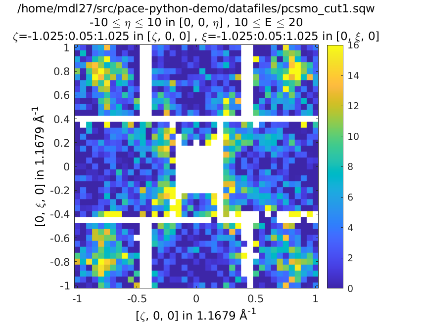
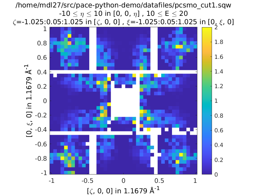
Left is the data, right is the calculation with resolution convolution.

Generic interface

As we saw from the examples above, the Horace multifit application expects a model function to have the following signature:

I = function user_model(qh, qk, ql, en, parameters, varargin)

where qh, qk, ql, and en are \(n_{\mathrm{pix}}\)-length vectors denoting the coordinates of the pixels of a Horace sqw object, or the bin centres of a dnd object. The function should return an \(n_{\mathrm{pix}}\)-length vector I of neutron intensities at those coordinates. parameters is a vector of the current iteration’s fittable parameter values, and varargin is an optional cell array denoting a variable-length argument list, using standard Matlab syntax.

This function is passed to a multifit object using the set_fun method, and its initial parameters set using the set_pin method:

kk = multifit(ws);
kk = kk.set_fun(@user_model);
kk = kk.set_pin({parameters, varargin{:}});

If there are no arguments to be passed (e.g. varargin should be empty), then a vector rather a cell array can be passed to set_pin:

kk = kk.set_pin(parameters);

In the following sections we describe how user defined model functions in several different languages can be used with the multifit application in Horace. We will use the example of spin waves in bcc-Iron, where the scattering function is given by:

\[ \begin{align}\begin{aligned}S(q_h, q_k, q_l, E) &= \frac{I_0}{\pi} \frac{4\Gamma E_0}{(E^2 - E_0^2)^2 - 4(\Gamma E)^2} \mathcal{N} \mathcal{F}\\\begin{split}\\\end{split}\\E_0(q_h, q_k, q_l, E) &= \Delta + 8 J \left(1 - \cos(\pi q_h) \cos(\pi q_k) \cos(\pi q_l) \right)\\\mathcal{N}(E) &= \frac{E}{1 - \exp \left( - \frac{E}{k_B T} \right)}\\\mathcal{F}(q) &= A \exp(-a q^2) + B \exp(-b q^2) + C \exp(-c q^2) + D\end{aligned}\end{align} \]

where \(I_0\) is an amplitude (intensity scaling) parameter, \(\Gamma\) is an energy width parameter, \(\Delta\) is an energy gap parameter, and \(J\) is an exchange parameter to be fitted. Thus \(E_0(E)\) is the dispersion relation, \(\mathcal{N}_(T)\) is the thermal population (Bose) factor where \(k_B\) is Boltzmann’s constant and \(T\) the sample temperature. \(F(q)\) is the magnetic form factor for metallic iron with \(q = \sqrt{q_h^2 + q_k^2 + q_l^2}/(4a^2)\), where \(a=2.87~\text{Å}\) is the lattice parameter of bcc-Iron and the parameters \(A=0.0706\), \(a=35.008\), \(B=0.3589\), \(b=15.358\), \(C=0.5819\), \(c=5.561\), and \(D=-0.0114\).

The data file for the code examples below can be downloaded from here.

Matlab function

The simplest case is for a model function written in Matlab. Put the following into a file called fe_sqw.m:

function out = fe_sqw(h, k, l, e, p)

js = p(1); d = p(2); gamma = p(3); I0 = p(4); temperature = p(5);

E0 = d + (8*js) .* (1 - cos(pi * h) .* cos(pi * k) .* cos(pi * l));
q2 = (h.^2 + k.^2 + l.^2) ./ ((2*2.87)^2);

% The magnetic form factor of iron
A=0.0706; a=35.008;  B=0.3589; b=15.358;  C=0.5819; c=5.561;  D=-0.0114;
ff = A * exp(-a*q2) + B * exp(-b*q2) + C * exp(-c*q2) + D;

out = (ff.^2) .* (I0/pi) .* (e ./ (1-exp(-11.602*e/temperature))) ...
      .* (4 * gamma * E0) ./ ((e.^2 - E0.^2).^2 + 4*(gamma * e).^2);

For simplicity we have passed the sample temperature as a fit variable but it should be fixed in the fitting:

% Make a cut of the data
proj = projaxes([1,1,0], [-1,1,0], 'type', 'rrr');
w_fe = cut_sqw('fe_cut.sqw', proj, [-3,0.05,3], [-1.05,-0.95], [-0.05,0.05], [70, 90]);

% Define starting parameters
J = 35;     % Exchange interaction in meV
D = 0;      % Single-ion anisotropy in meV
gam = 30;   % Intrinsic linewidth in meV (inversely proportional to excitation lifetime)
temp = 10;  % Sample measurement temperature in Kelvin
amp = 300;  % Magnitude of the intensity of the excitation (arbitrary units)

% Define the fitting problem
kk = multifit_sqw(w_fe)
kk = kk.set_fun (@fe_sqw, [J, D, gam, amp, temp])
kk = kk.set_free ([1, 1, 1, 1, 0])
kk = kk.set_bfun (@linear_bg, [0.1, 0])
kk = kk.set_bfree ([1, 0])

[wfit, fitdata] = kk.fit()
plot(w_fe); pl(wfit);

Note that we have used an alternative syntax for set_fun where the initial parameter is also set and then forced the sample temperature (the 5th parameter) to be fixed during the fitting with kk = kk.set_free([1,1,1,1,0]).

Alternatively we could have defined the function to take the temperature as an extra argument and only have 4 fittable parameters:

function out = fe_sqw(h, k, l, e, p, temperature)
js = p(1); d = p(2); gamma = p(3); I0 = p(4);

Then the fitting code would be:

kk = multifit_sqw(w_fe)
kk = kk.set_fun (@fe_sqw, {[J, D, gam, amp] temp})

Python function

If your model function is defined in Python, or requires the use of Python modules, it is still possible to call it in Horace using the in-built Python calling facility of Matlab. This is accessed using the py. namespace.

For example, let us define a Python file called fe_module.py with the following function:

import numpy as np

def fe_function(h, k, l, e, p, temperature):
    js = p[0]; d = p[1]; gamma = p[2]; I0 = p[3]
    E0 = d + (8*js) * (1 - np.cos(np.pi * h) * np.cos(np.pi * k) * np.cos(np.pi * l))
    q2 =  (h**2 + k**2 + l**2) / ((2*2.87)**2)
    # The magnetic form factor of iron
    A=0.0706; a=35.008;  B=0.3589; b=15.358;  C=0.5819; c=5.561;  D=-0.0114;
    ff = A * np.exp(-a*q2) + B * np.exp(-b*q2) + C * np.exp(-c*q2) + D
    return (ff**2) * (I0/np.pi) * (e / (1-np.exp(-11.602*e/temperature))) \
           * (4 * gamma * E0) / ((e**2 - E0**2)**2 + 4*(gamma * e)**2)

Because multifit expects a Matlab function handle, we must now wrap this Python function in a Matlab anonymous function (equivalent to a Python lambda function):

fe_sqw_py = @(h,k,l,e,p,temperature) double(py.fe_module.fe_function( ...
             py.numpy.array(h), py.numpy.array(k), py.numpy.array(l), ...
             py.numpy.array(en), py.numpy.array(p)), temperature);
kk = multifit_sqw(w_fe)
kk = kk.set_fun (@fe_sqw_py, {[J, D, gam, amp] temp})
kk = kk.set_bfun (@linear_bg, [0.1, 0])
kk = kk.set_bfree ([1, 0])
[wfit, fitdata] = kk.fit();

C / C++ / Fortran function

Finally, we can also call compiled functions written in C, C++ or Fortran from Matlab but there are some limitations:

• We use the loadlibrary Matlab function, which expects a “C-style” shared library. This means that C++ functions must be declared with extern "C" and Fortran 90 functions must be declared with the bind(C) attribute (this means that Fortran 77 or earlier is not supported).

• This also means that the function must be compiled as a shared-object (.so) library (dynamically-linked library (.dll) in Windows).

• To ensure that there are no heap memory errors, and to avoid slow-downs in copying large arrays, the model function must use an pre-allocated array for the results and should not allocate any arrays itself to return to Matlab (e.g. C/C++ functions must return void and Fortran must functions must be declared as subroutine).

• To allow the same interface for C/C++ and Fortran, the C/C++ functions must pass by reference.

In addition, for the examples below we restrict to the case where no non-variable arguments are specified (e.g. the first Matlab example where the temperature is included in the set of “variable” parameters but is fixed by set_free). This is not a general restriction but including such a facility is complex and may not be needed in most cases. There is some discussion here of how this could be done, and the interested user should contact a Horace developer for further help.

Prerequisites

Like the Python model function described above, we need to have a Matlab wrapper function:

function out = compiled_model(h, k, l, en, p, libname, funcname)
    res = libpointer('doublePtr', h);
    if ~libisloaded(libname)
        temp_header = [tempname(), '.h'];
        fid = fopen(temp_header, 'w');
        fprintf(fid, ['void %s(const double *qh, const double *qk, const double *ql, ' ...
                      'const double *en, const double *parameters, double *result, ' ...
                      'int *n_elem);'], funcname);
        fclose(fid);
        loadlibrary(libname, temp_header);
    end
    calllib(libname, funcname, h, k, l, en, p, res, numel(h));
    out = res.value;
end

Put the above code into a file compiled_model.m. Note that:

• The function requires a libname which is the name of the compiled shared library (a .so file in Linux or .dll file in Windows) without the extension. This library file must be on the Matlab path.

• The Matlab loadlibrary function is used to automatically load the library so it is not necessary for you to manually load it.

• The Matlab libpointer function is used to create an empty array res to hold the calculated intensity from the function.

• Because the compiled function is passed as pointers to the arrays, it needs to know their size, hence the final argument in the call to calllib is numel(h), the number of array elements.

C example

#include <math.h>

void fe_c_func(const double *qh, const double *qk, const double *ql, const double *en,
               const double *parameters, double *result, int *n_elem)
{
    const double js = parameters[0];
    const double d = parameters[1];
    const double gam = parameters[2];
    const double amp = parameters[3] / M_PI;
    const double tt = parameters[4];
    const double js8 = 8 * js;
    const double qscal = pow(1./(2.*2.87), 2.);
    const double A=0.0706, a=35.008, B=0.3589, b=15.358, C=0.5819, c=5.561, D=-0.0114;

    double E0, q2, ff, e2E02, game;
    for (int i=0; i<*n_elem; i++) {
        E0 = d + js8 * (1. - cos(M_PI * qh[i]) * cos(M_PI * qk[i]) * cos(M_PI * ql[i]));
        q2 = qscal * (qh[i]*qh[i] + qk[i]*qk[i] + ql[i]*ql[i]);
        ff = A * exp(-a * q2) + B * exp(-b * q2) + C * exp(-c * q2) + D;
        e2E02 = (en[i]*en[i] - E0*E0);
        game = gam * en[i];
        result[i] = (ff * ff) * amp * (en[i] / (1 - exp(-11.602*en[i] / tt)))
                    * (4 * gam * om) / (e2E02*e2E02 + 4 * game * game);
    }

}

Put the above code into a file called fe_sqw.c and compile it with:

gcc -shared -o fe_sqw_c.so fe_sqw.c

Put the compiled library file into a folder on the Matlab path, and run the fit with:

kk = multifit_sqw(w_fe)
kk = kk.set_fun (@compiled_model, {[J, D, gam, amp, temp], 'fe_sqw_c', 'fe_c_func'})
kk = kk.set_free ([1, 1, 1, 1, 0])
kk = kk.set_bfun (@linear_bg, [0.1, 0])
kk = kk.set_bfree ([1, 0])
[wfit, fitdata] = kk.fit();

C++ example

Create a file fe_sqw.cpp with:

#include <cmath>

extern "C" {

void fe_cpp_func(const double *qh, const double *qk, const double *ql, const double *en,
                 const double *parameters, double *result, int *n_elem)
{
    const double js = parameters[0];
    const double d = parameters[1];
    const double gam = parameters[2];
    const double amp = parameters[3] / M_PI;
    const double tt = parameters[4];
    const double js8 = 8 * js;
    const double qscal = pow(1./(2.*2.87), 2.);
    const double A=0.0706, a=35.008, B=0.3589, b=15.358, C=0.5819, c=5.561, D=-0.0114;

    double E0, q2, ff, e2E02, game;
    for (int i=0; i<*n_elem; i++) {
        E0 = d + js8 * (1. - cos(M_PI * qh[i]) * cos(M_PI * qk[i]) * cos(M_PI * ql[i]));
        q2 = qscal * (qh[i]*qh[i] + qk[i]*qk[i] + ql[i]*ql[i]);
        ff = A * exp(-a * q2) + B * exp(-b * q2) + C * exp(-c * q2) + D;
        e2E02 = (en[i]*en[i] - E0*E0);
        game = gam * en[i];
        result[i] = (ff * ff) * amp * (en[i] / (1 - exp(-11.602*en[i] / tt)))
                    * (4 * gam * E0) / (e2E02*e2E02 + 4 * game * game);
    }

}

} // extern "C"

Compile it using:

g++ -shared -o fe_sqw_cpp.so fe_sqw.cpp

Put the compiled library file into a folder on the Matlab path, and run the fit with the same script as above, except that the function is now:

kk = kk.set_fun (@compiled_model, {[J, D, gam, amp, temp], 'fe_sqw_cpp', 'fe_cpp_func'})

Fortran example

Create a file fe_sqw.f90 with:

subroutine fe_f90_func(qh, qk, ql, en, parameters, results, n_elem) bind(C)
    implicit none
    real(8), parameter :: PI = 3.1415926535897932385

    real(8), dimension(n_elem), intent(in) :: qh, qk, ql, en
    real(8), dimension(5), intent(in) :: parameters
    real(8), dimension(n_elem), intent(out) :: results
    integer, intent(in) :: n_elem
    real(8) js, d, gam, tt, amp, qscal
    real(8) E0, q2, ff, e2E02, game
    real(8), parameter :: A = 0.0706, aa=35.008, B=0.3589, bb=15.358
    real(8), parameter :: C=0.5819, cc=5.561, DD=-0.0114
    integer :: i

    js = parameters(1) * 8
    d = parameters(2)
    gam = parameters(3)
    tt = parameters(4)
    amp = parameters(5) / PI
    qscal = (1. / (2. * 2.87))**2

    do i=1, n_elem
        E0 = d + js * (1. - cos(PI * qh(i)) * cos(PI * qk(i)) * cos(PI * ql(i)));
        q2 = qscal * (qh(i)*qh(i) + qk(i)*qk(i) + ql(i)*ql(i));
        ff = A * exp(-aa * q2) + B * exp(-bb * q2) + C * exp(-cc * q2) + DD;
        e2E02 = (en(i)*en(i) - E0*E0);
        game = gam * en(i);
        results(i) = (ff * ff) * amp * (en(i) / (1 - exp(-11.602*en(i) / tt))) &
                     * (4 * gam * E0) / (e2E02*e2E02 + 4 * game * game);
    end do

end subroutine user_model_sqw

Compile it using:

gfortran -shared -o fe_sqw_f90.so fe_sqw.f90

Put the compiled library file into a folder on the Matlab path, and run the fit with the same script as above, except that the function is now:

kk = kk.set_fun (@compiled_model, {[J, D, gam, amp, temp], 'fe_sqw_f90', 'fe_f90_func'})