Horace Diagnostics
This tutorial was originally a script designed to explore some of the diagnostic features in Horace that allow you to understand strange features in your data.
Whole script available here.
This will take you through all the steps from generation, spurion spotting, and analysis.
Generating the data
%Take a cut from an sqw file, to get a dispersion plot. Ensure we
% do not %select the -nopix option. While this means that the object
% "cs" will be larger in memory than with `-nopix`.
% It will retain all of the information about detector pixels from
% individual runs (sample orientations) during the experiment.

sqw_file='/mnt/data/Science/URu2Si2/data/sqw/Ei81_20K.sqw';

proj = line_proj([1, 0 ,0], [0, 1, 0]);

cs=cut(sqw_file,proj,[-0.05,0.05],[-4,0.04,-2],[-0.05,0.05], [0,0.8,20]);

%Plot this:
% we use the "compact" routine to ensure we get tight axes around the data,
% without too much white space
plot(compact(cs));

lz 0 100;
keep_figure;
Taking cut from data in file /mnt/data/Science/URu2Si2/data/sqw/Ei81_20K.sqw...
Step 1 of 1; Have read data for 488866 pixels -- now processing data... -----> retained 24161 pixels
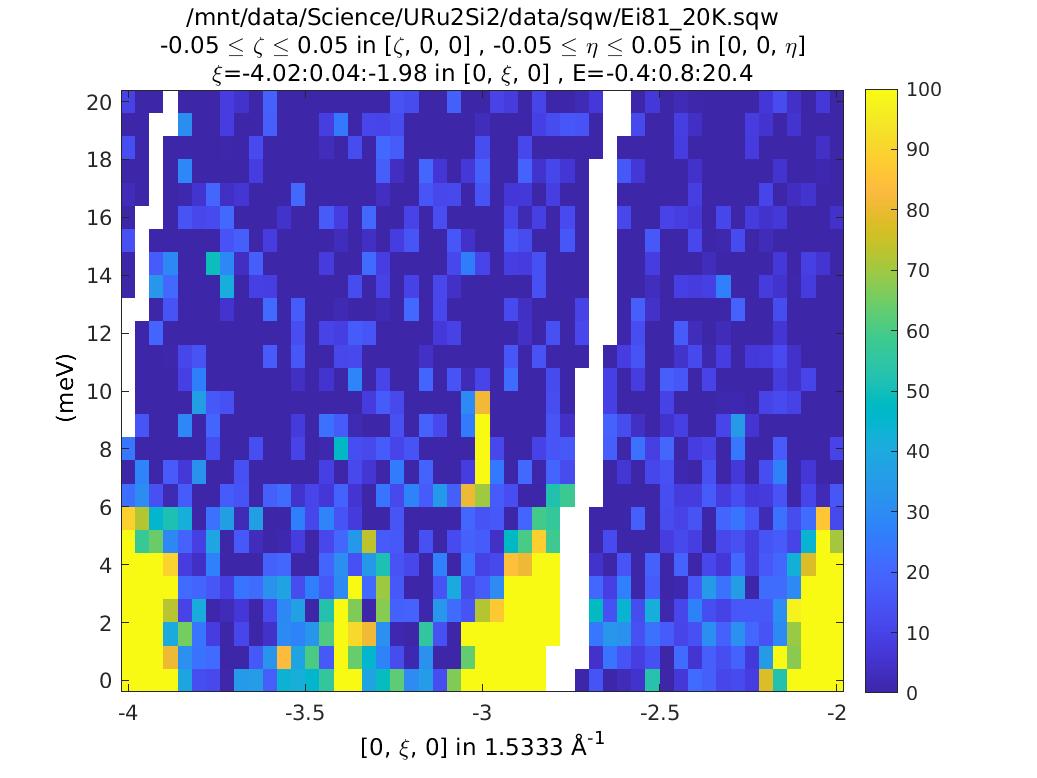
This is not very exciting, but notice there is an intense streak at K=-3, E=8. Is this real, or a spurion? One way to find out is to use the run inspector tool. This plots out the contributions to a cut from each of the individual runs (so long as you retained the detector pixel info, as we have here).
Run inspector
%Invoke the run inspector:
run_inspector(cs,'ax',[-4,-2,0,20],'col',[0,100]);
Note
The option ax sets the limits of the plot as follows: [xmin,
xmax, ymin, ymax].
If you don’t do this, then data from each run will be plotted with different axes, which makes them quite hard to compare.
Note
The option col sets the colourmap scale [col_min,col_max]. Again,
not setting this means data from each run will be plotted with
different colour scale, which is not so useful.
Note
You can explore the data, toggling between runs using the arrow keys, and using the page-up / page-down keys to skip 10 runs ahead.
Notice that the value of psi and the run number from when you made the data file are given in the plot title.
You should find that run 14 (psi=26) has a high point in the region we’re worried about. But runs 89 and 90 (psi=25 and 26), 150 (psi=26.5) and 209 (psi=25.5) do not have this feature.
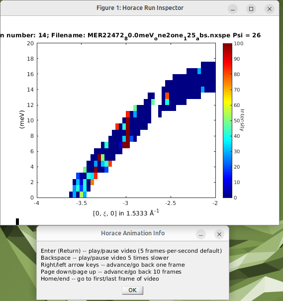
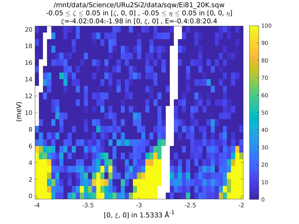
This suggests that it is a spurion. We can test this by masking the data just from this run in our object:
Note
the 14 here corresponds to the 14th run in our complete dataset
cs_m = mask_runs(cs,14);
plot(compact(cs_m));

keep_figure
and this confirms that indeed it was a spurion.
Understanding data from a single orientation
If you have a material which is strongly 1d or 2d you may well only measure with the sample in a single orientation. You can then integrate between +/- infinity on the axes where there is no dispersion. This improves statistics without the need to count lots of different orientations and hence is much faster.
Generating data
Generate a suitable sqw file, from a single orientation (see Taylor et al for an explanation of the science of this particular material).
Note
Below is an old style .spe file, so we need to supply a
.par file that gives info about the angular positions of the
detector elements. For modern .nxspe files this information is
already included and the par argument to gen_sqw can be an
empty string.
spe_file='/mnt/data/Science/Cs245/data/MER11499_one2one_113.spe';
par_file='/usr/local/mprogs/InstrumentFiles/trunk/merlin/one2one_113.par';

alatt=[2.8,2.8,7.7];
angdeg=[90,90,90];
psi=-90;  %single orientation

u=[1,1,0];
v=[0,0,1];

sqw_file2='/mnt/data/Science/Cs245/data/CsFeSe.sqw';
omega=0;
dpsi=0;
gl=0;
gs=0;

gen_sqw(spe_file,par_file,sqw_file2,40,1,alatt,angdeg,u,v,psi,omega,dpsi,gl,gs);

%Take a cut to show how the data look:
ccs=cut(sqw_file2,proj,[-1,0.02,1],[0.25,0.35],[-Inf,Inf],
[0,0.8,40]);
plot(ccs)
lz 0 20
keep_figure
--------------------------------------------------------------------------------
Calculating limits of data for 1 spe files...
Time to compute limits:
Elapsed time is 0.25054 seconds
 CPU time is 0.26 seconds
--------------------------------------------------------------------------------
Creating output sqw file:
Time to read spe and detector data:
Elapsed time is 14.5507 seconds
 CPU time is 14.86 seconds
Calculating projections...
Time to convert from spe to sqw data:
Elapsed time is 0.32091 seconds
 CPU time is 0.53 seconds
--------------------------------------------------------------------------------
Taking cut from data in file /mnt/data/Science/Cs245/data/CsFeSe.sqw...
Step 1 of 1; Have read data for 6672330 pixels -- now processing data... -----> retained 316821 pixels
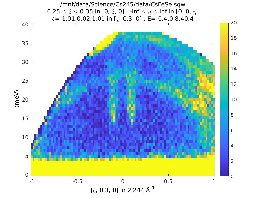
coordinates_calc
There is a routine in Horace called coordinates_calc, in which the
signal array in your data object is replaced by a value corresponding
to a Q or energy coordinate. Here we plot L (the direction we’ve
integrated along +/- inf here) to see what the value is explicitly as
we go up in energy
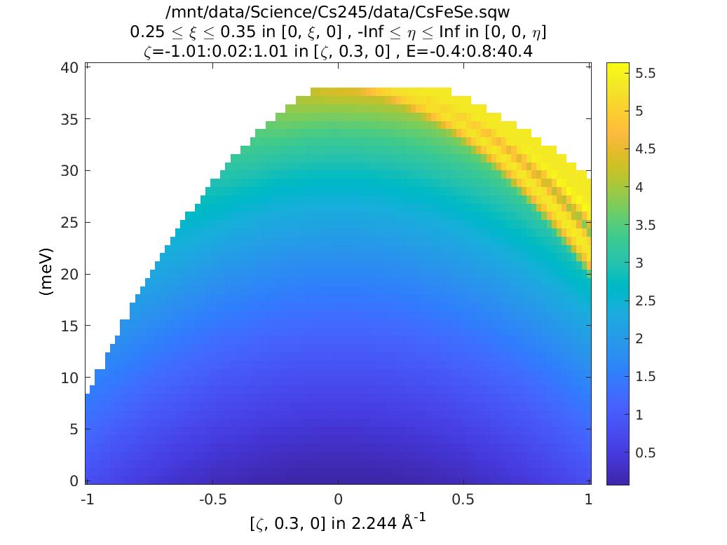
ccs_L = coordinates_calc(ccs,'L');
plot(ccs_L)
keep_figure
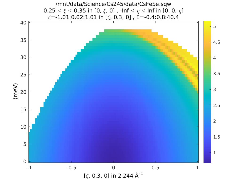
Notice that L is coupled to energy transfer. So this means as we increase energy we increase L, and hence \(\left|Q\right|\), which means the signal will be decreased due to the magnetic form factor.
%Can see this alternatively by plotting |Q|
ccs_Q = coordinates_calc(ccs,'Q');
plot(ccs_Q)
keep_figure
hkle
We can also get a list of h,k,l and e explicitly for a set of coordinates:
Note
Here the 2nd argument is of the form [x1,y1; x2,y2; x3,y3;….]
[qe1,qe2] = hkle(ccs,[0.11 14; 0.11 18; 0.11 22; 0.11 26; 0.11 30; 0.11 34]);
>> qe1

qe1 =

0.1100 0.3000 1.1332 14.0000
0.1100 0.3000 1.4891 18.0000
0.1100 0.3000 1.8809 22.0000
0.1100 0.3000 2.3225 26.0000
0.1100 0.3000 2.8396 30.0000
0.1100 0.3000 3.4932 34.0000

>> qe2

qe2 =

0.1100 0.3000 9.6355 14.0000
0.1100 0.3000 9.2796 18.0000
0.1100 0.3000 8.8878 22.0000
0.1100 0.3000 8.4462 26.0000
0.1100 0.3000 7.9291 30.0000
0.1100 0.3000 7.2755 34.0000
This tells us the values of h,k,l and e. As we saw above, the value of
L changes as we increase energy (qe1). But what is qe2? This
is the 2nd root, and corresponds to an alternative value of L that
could also contribute to the data here.
Putting it all together
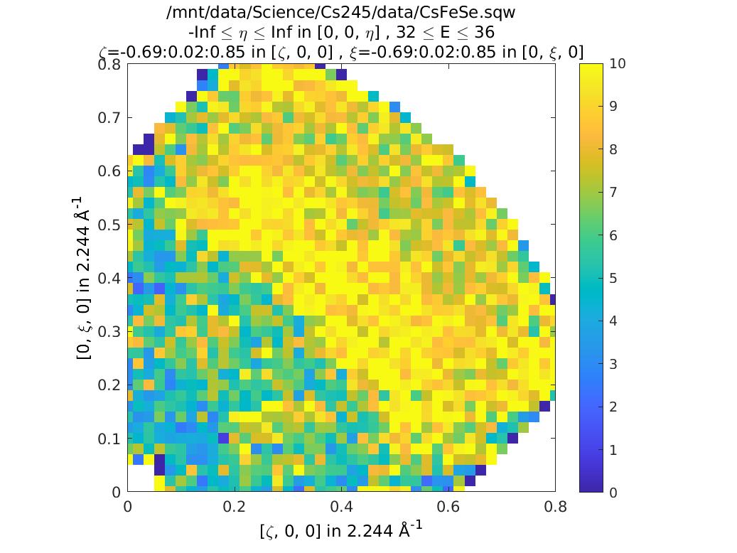
To understand what this means let’s plot a couple of constant energy slices:
ccs2 = cut(sqw_file2,proj,0.02,[0.25,0.35],0.05,[32,36]);
plot(compact(ccs2))
lz 0 20
keep_figure

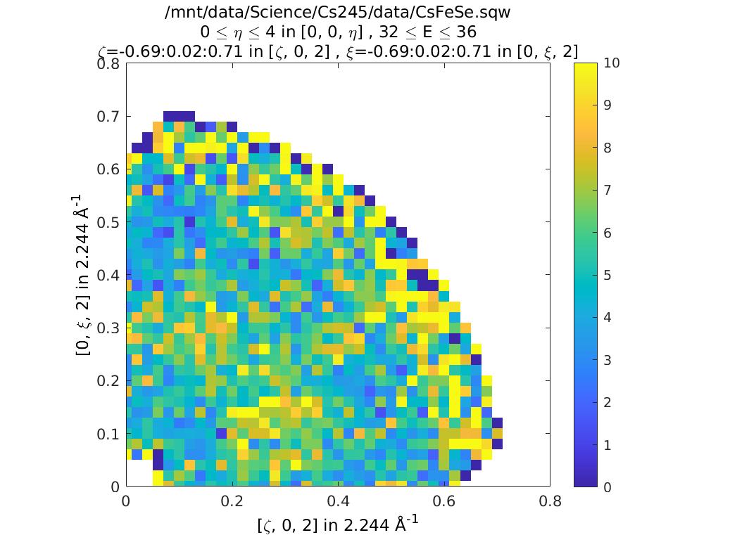
ccs3 = cut(sqw_file2,proj,0.02,0.02,[-Inf,Inf],[32,36]);
plot(compact(ccs3))
lz 0 10
lx 0 0.8
ly 0 0.8
Taking cut from data in file /mnt/data/Science/Cs245/data/CsFeSe.sqw...
Step 1 of 1; Have read data for 6672330 pixels -- now processing data... -----> retained 73281 pixels
Taking cut from data in file /mnt/data/Science/Cs245/data/CsFeSe.sqw...
Step 1 of 1; Have read data for 6672330 pixels -- now processing data... -----> retained 635460 pixels
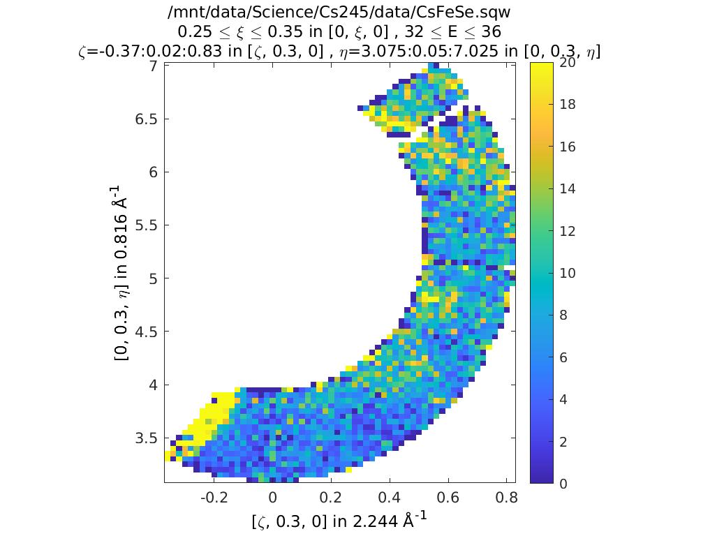
In the first of these slices, ccs2, we’ve changed the plot axes to be H
and L. You can see that the detectors describe a curved path in the H,L
plane, so for a given H, if we integrate between +/- infinity then we
might also pick up info from a much higher 2-theta.
In this case you can see this starts to become a problem for this particular MERLIN dataset around \(H > 0.35\).
The second slice, ccs3, illustrates this in practice. You can see that
at \(Q=(0.35,0.3)\) there is a step increase in the signal. This is
because we suddenly start to fold in the data from higher Q (phonon
signal).
To avoid this, we can set the limits of L in our original slice explicitly. Generally the workflow here is to do the integration between +/- infinity, and then figure out where in L you start to get a problem, and then restrict the range of L to avoid this:
ccs4 = cut(sqw_file2,proj,0.02,0.02,[0,4],[32,36]);
plot(compact(ccs4))
lz 0 10
lx 0 0.8
ly 0 0.8
keep_figure
Taking cut from data in file /mnt/data/Science/Cs245/data/CsFeSe.sqw...
Step 1 of 1; Have read data for 6672330 pixels -- now processing data... -----> retained 315307 pixels
Whole script
%Take a cut from an sqw file, to get a dispersion plot. Ensure we do not
%select the -nopix option, i.e. the object "cs" will be larger in memory,

%but will retain all of the information about detector pixels from
%individual runs (sample orientations) during the experiment.

sqw_file='/mnt/data/Science/URu2Si2/data/sqw/Ei81_20K.sqw';

proj = line_proj([1, 0 ,0], [0, 1, 0]);

cs=cut(sqw_file,proj,[-0.05,0.05],[-4,0.04,-2],[-0.05,0.05], [0,0.8,20]);

%Plot this:
%we use the "compact" routine to ensure we get tight axes around the data, without too much white space
plot(compact(cs));

lz 0 100;
keep_figure;

%Invoke the run inspector:
run_inspector(cs,'ax',[-4,-2,0,20],'col',[0,100]);

%We can test this by masking the data just from this run in our object
%the 14 here corresponds to the 14th run in our complete dataset
cs_m = mask_runs(cs,14);
plot(compact(cs_m));


spe_file='/mnt/data/Science/Cs245/data/MER11499_one2one_113.spe';
par_file='/usr/local/mprogs/InstrumentFiles/trunk/merlin/one2one_113.par';

alatt=[2.8,2.8,7.7];
angdeg=[90,90,90];
psi=-90;  %single orientation

u=[1,1,0];
v=[0,0,1];

sqw_file2='/mnt/data/Science/Cs245/data/CsFeSe.sqw';
omega=0;
dpsi=0;
gl=0;
gs=0;

gen_sqw(spe_file,par_file,sqw_file2,40,1,alatt,angdeg,u,v,psi,omega,dpsi,gl,gs);

%Take a cut to show how the data look:
ccs=cut(sqw_file2,proj,[-1,0.02,1],[0.25,0.35],[-Inf,Inf],
[0,0.8,40]);
plot(ccs)
lz 0 20
keep_figure


ccs_L = coordinates_calc(ccs,'L');
plot(ccs_L)
keep_figure

%Can see this alternatively by plotting |Q|
ccs_Q = coordinates_calc(ccs,'Q');
plot(ccs_Q)
keep_figure

% Here the 2nd argument is of the form [x1,y1; x2,y2; x3,y3;....]
[qe1,qe2] = hkle(ccs,[0.11 14; 0.11 18; 0.11 22; 0.11 26; 0.11 30; 0.11 34]);


% Cut a couple of constant energy slices

ccs2 = cut(sqw_file2,proj,0.02,[0.25,0.35],0.05,[32,36]);
plot(compact(ccs2))
lz 0 20
keep_figure

ccs3 = cut(sqw_file2,proj,0.02,0.02,[-Inf,Inf],[32,36]);
plot(compact(ccs3))
lz 0 10
lx 0 0.8
ly 0 0.8

ccs4 = cut(sqw_file2,proj,0.02,0.02,[0,4],[32,36]);
plot(compact(ccs4))
lz 0 10
lx 0 0.8
ly 0 0.8
keep_figure