How To Use ResINS To Find Optimal Experimental Settings
The data stored within ResINS can also be leveraged to plan INS experiments. One aspect of this is determining the optimal settings to use for an experiment. This guide aims to show the steps required to write a script that uses ResINS for this purpose, but please note:
Important
while this guide guarantees that the code will be correct, it cannot provide specific scientific guidance for any given scientific question. Some general advice is given, but consult a domain-area expert for any science concerns. Different experiments will require different considerations.
Using resolution plots
The optimal experimental settings can be estimated using purely ResINS and a plotting library, though some knowledge of the system under investigation is still required. To do this, the instrument, the model, and the option for each configuration have to have been chosen. The first step is to create the instrument:
>>> from resins import Instrument
>>> maps = Instrument.from_default('MAPS')
>>> print(maps)
Instrument(name=MAPS, version=MAPS)
and then find the settings and their defaults:
>>> data = maps.get_model_data('PyChop_fit')
>>> data.defaults
{'e_init': 500, 'chopper_frequency': 400}
which can be used as a starting point to generate some resolution data:
>>> import numpy as np
>>> model = maps.get_resolution_function('PyChop_fit', chopper_package='B')
>>> points = np.arange(0, data.defaults['e_init'], 0.5)[:, None]
>>> resolution = model.get_characteristics(points)['sigma']
Plotting with matplotlib:
import matplotlib.pyplot as plt

fig, ax = plt.subplots(figsize=(10, 6))

ax.plot(points[:, 0], resolution)

ax.set_xlabel('Energy transfer (meV)', fontsize=20)
ax.set_ylabel('Sigma (meV)', fontsize=20)
ax.tick_params(labelsize=14)

plt.show()
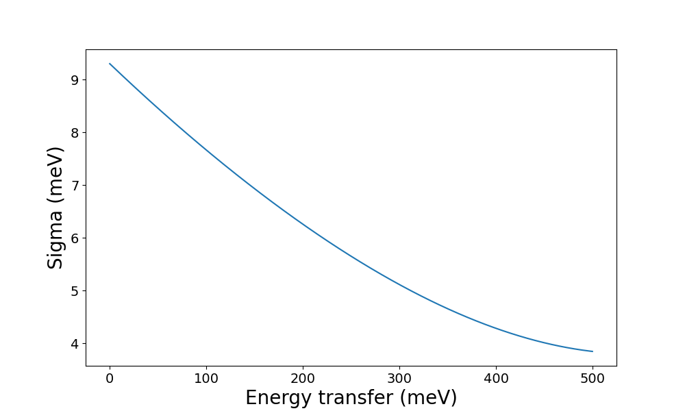
From here it should be possible to get an idea of the instrument properties and check whether the other choices (e.g. configuration) seem reasonable. If so, the next step is to plot the resolution at different combinations of the settings:
>>> data.restrictions
{'e_init': [0, 2000], 'chopper_frequency': [50, 601, 50]}
The restrictions provide information about the allowed values for each
setting. In the case of the MAPS instrument, there are two
settings:
e_initfor which all values between0and2000meV are allowedchopper_frequencyfor which values50,100,150, … are allowed up to600Hz.
Scientific constraints may also apply. For example, the direct-geometry instrument
MAPS can only observe values of energy transfer up to the incident energy (e_init).
If we intend to investigate spectral features between 100 and 600 meV, the useful e_init settings are limited to values above 600 meV:
>>> max_feature = 600
>>> test_e_init = np.arange(max_feature, max(data.restrictions['e_init']), 100)
>>> test_choppers = np.arange(*data.restrictions['chopper_frequency'])
All the data can then be generated using by loopiing over these variables:
>>> energy_transfer = np.arange(0, max_feature, 5)
>>> results = np.zeros((len(test_choppers), len(test_e_init), len(energy_transfer)))
>>> for i, chopper_frequency in enumerate(test_choppers):
...     for j, e_init in enumerate(test_e_init):
...         model = maps.get_resolution_function('PyChop_fit', chopper_package='B', e_init=e_init, chopper_frequency=chopper_frequency)
...         results[i, j, :] = model.get_characteristics(energy_transfer)['sigma']
This can then be plotted in various ways. For example, we can check the effect
of e_init by plotting the resolution for its different values at a constant
chopper_frequency, e.g. the default of 400 Hz:
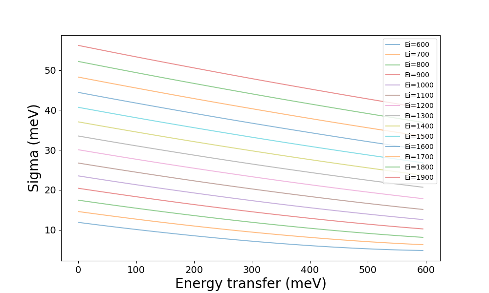
from which we might conclude that a low value for e_init is desirable, so we
might follow up by comparing the different values of chopper_frequency at
the lowest value of e_init, 600:
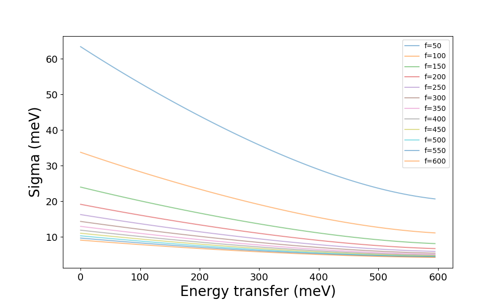
which might suggest that chopper_frequency of 300 Hz and above gives
tolerable resolution. Then, if the features are expected to be further apart
than the resolution, they should be distinguishable in an INS experiment. If
that is not the case, it might mean that this combination of instrument,
configurations, and settings
is unsuitable.
Using simulated spectra
The other way to estimate the optimal experimental settings is to simulate spectra from ab initio lattice dynamics or molecular dynamics, e.g. using AbINS or dynasor, and then convolve the ResINS resolution using a library like euphonic. Again, we begin by creating the Instrument:
>>> from resins import Instrument
>>> maps = Instrument.from_default('MAPS')
>>> print(maps)
Instrument(name=MAPS, version=MAPS)
and getting settings and their defaults:
>>> data = maps.get_model_data('PyChop_fit')
>>> data.defaults
{'e_init': 500, 'chopper_frequency': 400}
The defaults can be used as the starting point:
However, before proceeding, the computational data has to be loaded (here
represented using np.load but this will depend on the origin of the data):
after which euphonic can be used to broaden the spectrum:
as well as plot it: