Quick Start

With the package installed, the first step is to create an instance of a particular version of a particular instrument:

>>> from resins import Instrument
>>> maps = Instrument.from_default('MAPS', 'MAPS')
>>> print(maps)
Instrument(name=MAPS, version=MAPS)

To get the resolution function, a couple choices might be necessary:

Choose the model for our instrument.
Select one of the options for each configuration of the chosen model.
Provide any other settings that the model requires.

If we don’t know what the possibilities are for the chosen instrument, the information can be found either in the documentation or programmatically:

>>> maps.available_models
['PyChop_fit']
>>> maps.get_model_signature('PyChop_fit')
<Signature (model_name: Optional[str] = 'PyChop_fit_v1', *, chopper_package: Literal['A', 'B', 'S'] = 'A', e_init: Annotated[ForwardRef('Optional[float]'), 'restriction=[0, 2000]'] = 500, chopper_frequency: Annotated[ForwardRef('Optional[int]'), 'restriction=[50, 601, 50]'] = 400, fitting_order: 'int' = 4, _) -> resins.models.pychop.PyChopModelFermi>

With this, it is possible to make the choices and obtain the resolution function via the get_resolution_function() method:

>>> pychop = maps.get_resolution_function('PyChop_fit', chopper_package='B', e_init=500, chopper_frequency=300)
>>> print(pychop)
PyChopModelFermi(citation=['R. I. Bewley, R. A. Ewings, M. D. Le, T. G. Perring and D. J. Voneshen, 2018. PyChop', 'https://mantidproject.github.io/docs-versioned/v6.10.0/interfaces/direct/PyChop.html'])

Note

The settings and configurations must be passed in as keyword arguments.

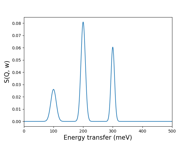
The obtained model can be called (like a function) to broaden data at the provided combinations of energy transfer and momentum ([w, Q]), using a mesh and the corresponding data:

>>> import numpy as np
>>> energy_transfer = np.array([100, 200, 300])[:, np.newaxis]
>>> data = np.array([0.6, 1.5, 0.9])
>>> mesh = np.linspace(0, 500, 1000)
>>> result = pychop(energy_transfer, data, mesh)

which can be plotted as:

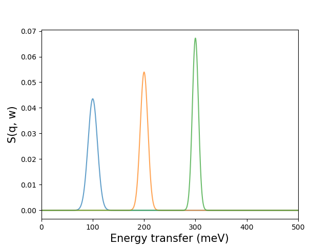
However, the model also provides methods for more fundamental operations: get_kernel computes the broadening kernel at each [w, Q] (centered on 0), get_peak computes the broadening peak at each [w, Q] (centered on the [w, Q]), and get_characteristics returns only the characteristic parameters of the kernel at each [w, Q] (such as the standard deviation of the normal distribution):

>>> pychop.get_characteristics(energy_transfer)
{'sigma': array([9.15987016, 7.38868127, 5.93104319])}
>>> peaks = pychop.get_peak(energy_transfer, mesh)

Can be plotted as:

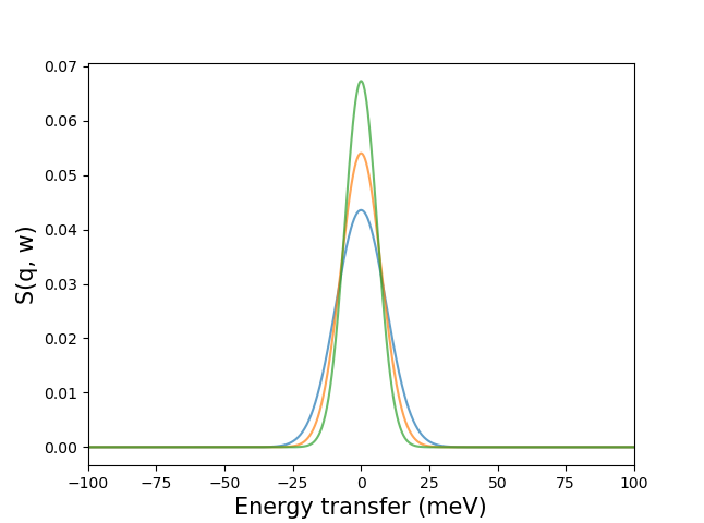
>>> mesh_centered_on_0 = np.linspace(-100, 100, 1000)
>>> kernels = pychop.get_kernel(energy_transfer, mesh_centered_on_0)

Can be plotted as: