dnd vs sqw: the difference
This tutorial was originally a script designed to illustrate and explain the
different key data types – sqw and dnd (the d0d, ``d1d`, …
family). – in Horace, and why they are important.
Whole script available here.
The key difference is that sqw objects contain the exact data for each
measurement (pixels) while dnd objects simply contain the histogrammed
(binned) accumulation of these data.
For more information on the differences between dnd and sqw, see
here.
%Take two cuts:
sqw_file='/mnt/data/Science/URu2Si2/data/sqw/Ei81_20K.sqw';

proj = line_proj([1, 0, 0], [0, 1, 0]);

csqw=cut(sqw_file, proj, [-0.5, 0.5], [-4, 0.04, -2], [-0.05, 0.05], [0, 0.8, 60]);

%identical to above, except extra argument at the end
cdnd=cut(sqw_file, proj, [-0.5, 0.5], [-4, 0.04, -2], [-0.05, 0.05], [0, 0.8, 60], '-nopix');

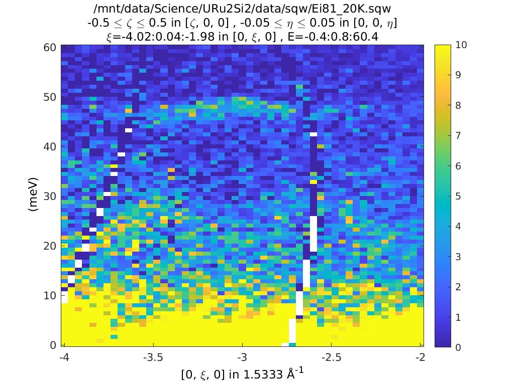
plot(compact(csqw));
lz 0 10;
keep_figure;

plot(compact(cdnd));
lz 0 10;
keep_figure;
Taking cut from data in file /mnt/data/Science/URu2Si2/data/sqw/Ei81_20K.sqw...
Step 1 of 1; Have read data for 5579774 pixels -- now processing data... -----> retained 1121852 pixels
Taking cut from data in file /mnt/data/Science/URu2Si2/data/sqw/Ei81_20K.sqw...
Step 1 of 1; Have read data for 5579774 pixels -- now processing data... -----> retained 1121852 pixels


The plots look (are!) identical. So what’s the difference? Double click on them
in the Workspace part of the Matlab window. You can see that the csqw object
has a lot more information associated with it.
General principle
Use dnd if you are just looking at the data - it takes up less computer
memory, which is a good thing.
If you want to fit or simulate the data and you are only simulating a
basic function (i.e. using func_eval, multifit_func, etc) that does not
depend on all 4 coordinates of Q and E, then use a dnd.
Example:
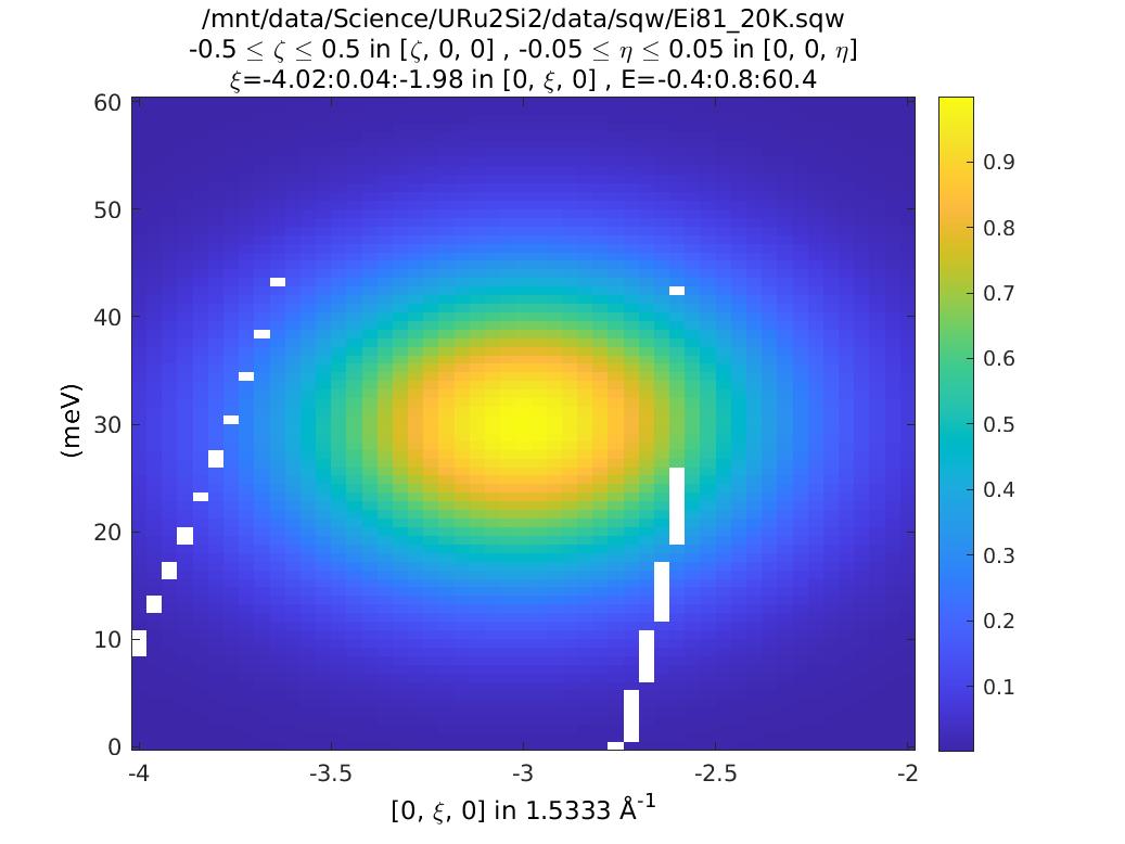
cgaussdnd=func_eval(cdnd, @gauss2d, [1, -3, 30, 0.2, 0.1, 100]);
plot(cgaussdnd);
keep_figure;

cgausssqw=func_eval(csqw, @gauss2d, [1, -3, 30, 0.2, 0.1, 100]);
plot(cgausssqw);
keep_figure;


The two figures are identical, because the func_eval routine only uses the plot axis coordinates as its input, not (H, K, L, E).
If you want to fit or simulate data with an S(Q, E) model, you should
use sqw. This is because you will account for the fact that you had to
integrate along the non-plot axes correctly. The following example illustrates
why this is important:
%model of ferromagnetic spin waves in the Horace demo
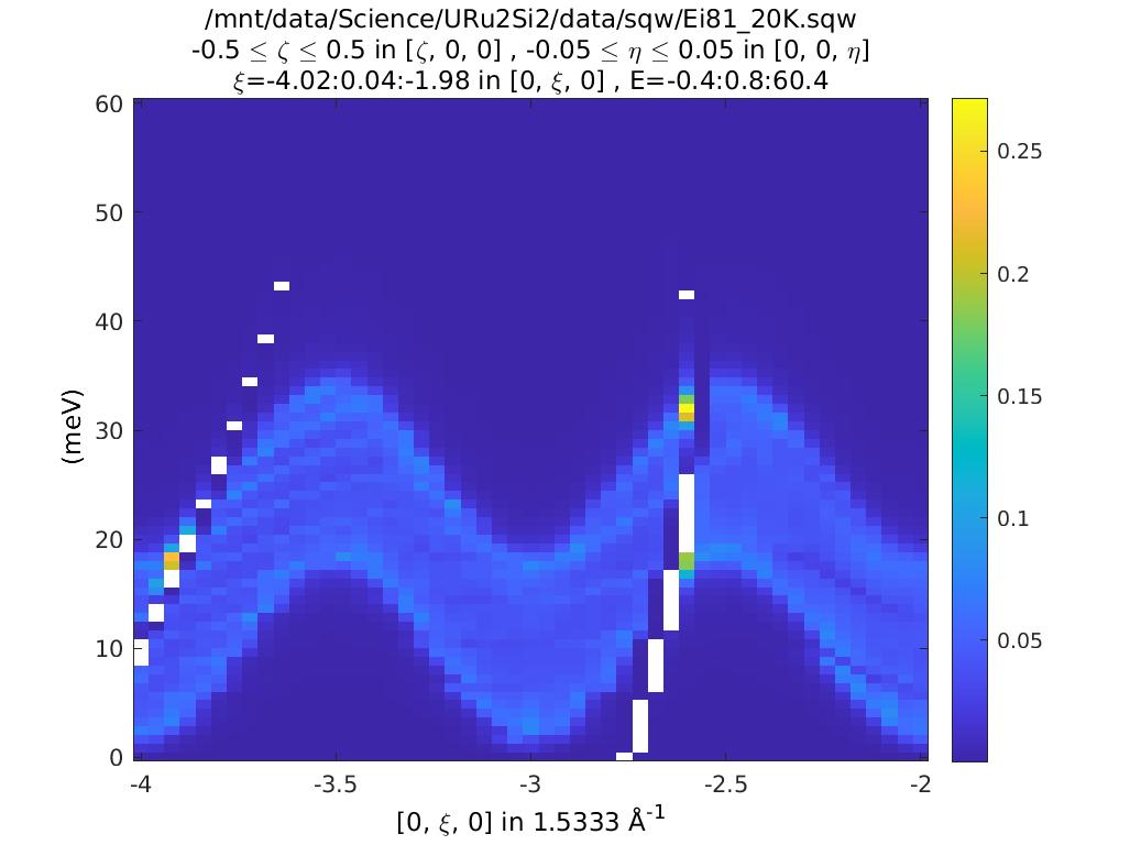
csimsqw=sqw_eval(csqw, @demo_FM_spinwaves_2dSlice_sqw, [4, 2, 1, 1, 1]);
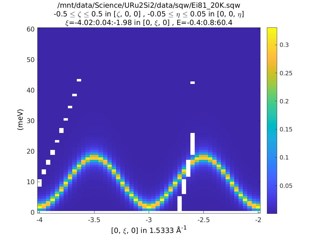
csimdnd=sqw_eval(cdnd, @demo_FM_spinwaves_2dSlice_sqw, [4, 2, 1, 1, 1]);

%Dispersion has equal steepness along all reciprocal space directions.
plot(csimsqw);
keep_figure;

plot(csimdnd);
keep_figure;


These are totally different.
Why?
Because the simulation of the sqw object includes the dispersion along the
H-axis, and calculates what it is for the pixels actually measured. The
simulation of the dnd object assumes that every point has the average value
of H (zero in this case). So the latter gives a sharp dispersion, whereas the
former is very broad.
So if you have data from a system where there is some variation in the signal
along a non-plot axis, you should use simulate with sqw objects in order
to capture this correctly.
Specific case A: resolution modelling
If you want to include resolution in your simulation or fitting, you must use
Tobyfit, and you also need the detector pixel information that you get in an
sqw object but not in a dnd.
Warning
Tobyfit will give an error message if you try to use it with a dnd.
Specific case B: spurion identification
See separate tutorial about how to do this. Basically, if you need to know
something about data from a particular run, or from a particular detector, you
need sqw.
Specific case C: smoothing
If you apply the smooth algorithm to your data you will get a dataset of the
same type back again. Smoothing works for dnd, but is forbidden for sqw
data. The reason is that the smoothing operation only makes sense in the plot
axis coordinate frame. But doing that means you lose the connection between the
signal displayed in the plot and the detector pixel information that contributed
to it.
Specific case D: symmetrisation
Warning
Currently in Horace 4.0.0, dnd symmetrisation is disabled. Due to
extended transforms in the sqw object.
Symmetrisation does different things for sqw and dnd data. The latter
can be folded along an axis parallel to a plot axis. The former can be folded
along any axis. Generally you are much safer doing symmetrisation with sqw
objects.
Whole Script
%Take two cuts:
sqw_file='/mnt/data/Science/URu2Si2/data/sqw/Ei81_20K.sqw';

proj = line_proj([1, 0, 0], [0, 1, 0]);

csqw=cut(sqw_file, proj, [-0.5, 0.5], [-4, 0.04, -2], [-0.05, 0.05], [0, 0.8, 60]);

%identical to above, except extra argument at the end
cdnd=cut(sqw_file, proj, [-0.5, 0.5], [-4, 0.04, -2], [-0.05, 0.05], [0, 0.8, 60], '-nopix');

plot(compact(csqw));
lz 0 10;
keep_figure;

plot(compact(cdnd));
lz 0 10;
keep_figure;

cgaussdnd=func_eval(cdnd, @gauss2d, [1, -3, 30, 0.2, 0.1, 100]);
plot(cgaussdnd);
keep_figure;

cgausssqw=func_eval(csqw, @gauss2d, [1, -3, 30, 0.2, 0.1, 100]);
plot(cgausssqw);
keep_figure;

%model of ferromagnetic spin waves in the Horace demo
csimsqw=sqw_eval(csqw, @demo_FM_spinwaves_2dSlice_sqw, [4, 2, 1, 1, 1]);
csimdnd=sqw_eval(cdnd, @demo_FM_spinwaves_2dSlice_sqw, [4, 2, 1, 1, 1]);

%Dispersion has equal steepness along all reciprocal space directions.
plot(csimsqw);
keep_figure;

plot(csimdnd);
keep_figure;