Using a pre-trained MLIP with Phonopy

For accurate results one would typically compute phonons with density-functional theory or with a system-specific interatomic potential. However, at the early stages of a project it may be useful to run a “general” machine-learned interatomic potential (MLIP) which is been trained on a variety of systems.

In this tutorial we primarily use the MACE-OFF23 [1] potential which is trained on organic molecules; the more general MACE-MP-0 [2] can be used in the same way for other chemistries. In both cases we are using the ASE Calculator interface; most popular MLIP packages have an ASE interface and so can be used in a similar fashion.

We will also use ASE for geometry optimisation and Phonopy for setting-up/post-processing the force-constant calculations.

This example workflow is implemented as a small Python program, with steps broken out into different functions. We will examine the functions separately in this document: to test the overall workflow you can run the program, or implement your own using the building blocks shown.

Step 0: setting up the machine-learned interatomic potential (MLIP)

First, we need to set up an MLIP implementation. Here we assume that the MACE package has already been installed into the current environment. (See: Environment setup.) Then we can create an ASE calculator, ready to attach to a structure (Atoms) object.

        from mace.calculators import mace_off

        calc = mace_off(model="medium", device=device, default_dtype="float64")

There are a range of MLIP packages available and most of them provide an ASE calculator, or have had one wrapped around them. Here are a few, in no particular order:

MLIP package	ASE interface
QUIP (GAP)	quippy
JuLIP (ACE)	pyjulip
MACE	Yes
pacemaker (ACE)	Yes
GPUMD (NEP)	calorine
NequIP	Yes
n2p2	via LAMMPS
SchNetPack	Yes

Step 1: geometry optimisation

First, we grab an input structure for hexane from the CCSD <https://doi.org/10.5517/cc3gcpl> in CIF format. Here the file provided by CCSD has already been converted to a simpler format and saved as a “geometry.in” file in the FHI-aims format. (As we will be using ASE, we can work with whichever format looks the nicest!)

We then optimise the geometry with a very fine force criterion, in order to get as close to the minimum-energy configuration as possible.

    atoms = ase.io.read(filename)
    atoms = get_optimized_geometry(atoms, calc)

def get_optimized_geometry(
    atoms: Atoms,
    calc: Calculator,
    trajectory_file: Path | str = "opt.traj",
    fire_steps=30,
    fmax=1e-6,
) -> Atoms:
    """Optimize geometry in two stages using ASE

    The FIRE optimiser is very stable, and can be a good starting point if we
    are starting far from the minimum-energy configuration. We then switch to
    the QuasiNewton optimiser which is more efficient when close to the minimum.

    Returns an optimised copy of the input atoms with calc attached.

    """

    atoms = atoms.copy()
    atoms.calc = calc

    traj = Trajectory(trajectory_file, "w", atoms)

    opt = FIRE(atoms)
    opt.attach(traj)
    opt.run(steps=fire_steps)

    opt = QuasiNewton(atoms)
    opt.attach(traj)
    opt.run(fmax=fmax)

    return atoms

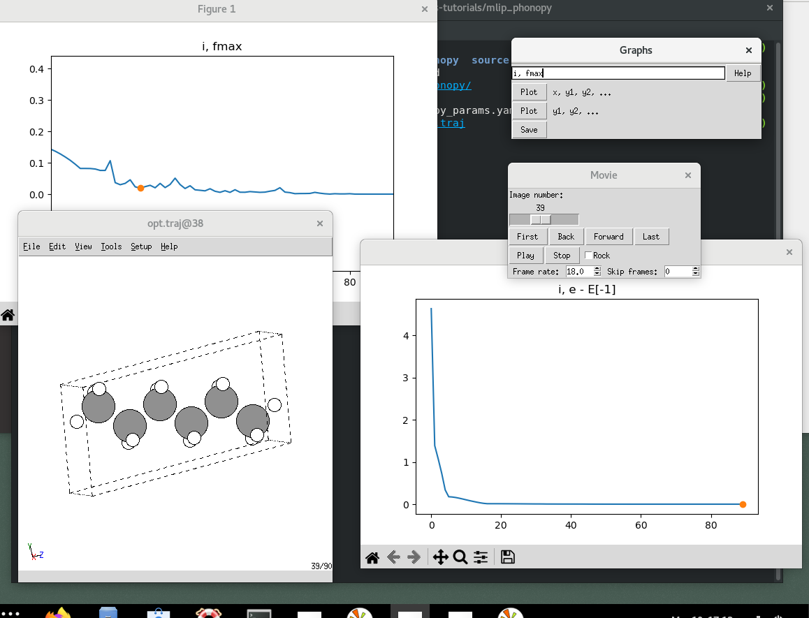
To get a sense of the optimisation progress, examine the trajectory file with

ase gui opt.traj

and create a plot of max forces by entering i, fmax in the Graphs window.

Step 2: finite displacements

We will use the Phonopy Python API to create supercells with displaced atoms and analyse the forces.

A few lines of code are needed to adapt between the ASE and phonopy structure representations: to keep things tidy we wrap these into functions.

def phonopy_from_ase(atoms: Atoms) -> PhonopyAtoms:
    """Convert ASE Atoms to PhonopyAtoms object"""
    return PhonopyAtoms(
        symbols=atoms.symbols,
        cell=atoms.cell,
        scaled_positions=atoms.get_scaled_positions(),
    )


def ase_from_phonopy(phonopy_atoms: PhonopyAtoms) -> Atoms:
    """Convert PhonopyAtoms to ASE Atoms object"""
    return Atoms(
        phonopy_atoms.symbols,
        cell=phonopy_atoms.cell,
        scaled_positions=phonopy_atoms.scaled_positions,
        pbc=True,
    )

Now we set up the displacements: the displaced structures are created on the Phonopy object as phonopy.supercells_with_displacements. SYMPREC (symmetry threshold) and DISP_SIZE (finite displacement distance) are parameters controlling the displacement scheme; in the sample program they are set to 1e-4 and 1e-3 respectively. The supercell matrix is another user parameter; this has a significant impact on the runtime and the quality of results, so should be checked carefully.

    # Phonopy uses its own ASE-like structure container
    phonopy = Phonopy(
        phonopy_from_ase(atoms), supercell_matrix=supercell, symprec=SYMPREC
    )
    phonopy.generate_displacements(distance=DISP_SIZE)

Step 3: force calculations

Using ASE the idiom for calculating forces on a structure is:

• attach a “calculator” to the structure atoms.calc = calculator

• call atoms.get_forces())

Here we do this for each of the displaced supercells, collecting the results into a list for later use. tqdm is used to make a nice progress bar while this runs; for large supercells it may take a while!

    force_container = []

    def _get_forces(atoms: Atoms) -> np.ndarray:
        atoms.calc = calc
        return atoms.get_forces()

    all_forces = [
        _get_forces(ase_from_phonopy(displaced_supercell))
        for displaced_supercell in tqdm(phonopy.supercells_with_displacements)
    ]

Step 4: constructing force constants

The force constants are the Hessian of our supercell, and can be used to generate phonon band structures and simulated neutron spectra.

We attach the calculated forces to the Phonopy object and instruct it to compute the force constants and write data files.

    phonopy.forces = all_forces
    phonopy.produce_force_constants()

    print(f"      Saving to files {PHONOPY_FILE} and force_constants.hdf5 ...")
    phonopy.save(filename=PHONOPY_FILE, settings={"force_constants": False})
    from phonopy.file_IO import write_force_constants_to_hdf5

    write_force_constants_to_hdf5(phonopy.force_constants)


if __name__ == "__main__":
    typer.run(main)

Here we write the force constants to a force_constants.hdf5 file. This is only recently supported by Abins; to include the force constants in the .yaml file instead use

phonopy.save(filename=PHONOPY_FILE, settings={"force_constants": True})

This is compatible with more versions of Abins, and more convenient as the file can have any name. However, the data loading may be noticeably slower as the YAML format is not designed for large numerical arrays.

Step 5: INS simulation with Abins Python interface

Plotting is implemented in a separate script abins_plot.py. After collecting the phonopy data filename and measurement temperature from the user we can call Abins:

    mantid.simpleapi.Abins(
        VibrationalOrPhononFile=str(filename),
        AbInitioProgram="FORCECONSTANTS",
        OutputWorkspace="abins-output",
        TemperatureInKelvin=temperature,
        SumContributions=True,
        ScaleByCrossSection="Total",
        QuantumOrderEventsNumber="2",
        Autoconvolution=True,
        Instrument="TOSCA",
        Setting="Backward (TOSCA)",
    )

Abins is an “Algorithm” in Mantid, and writes its results to Workspace objects. In a graphical Workspace session we can manage these from an interactive panel: from Python it can be useful to check our available workspaces using

mantid.simpleapi.AnalysisDataService.getObjectNames()

['abins-output',
 'abins-output_C_quantum_event_1',
 'abins-output_C_quantum_event_10',
 'abins-output_C_quantum_event_2',
 'abins-output_C_quantum_event_3',
 'abins-output_C_quantum_event_4',
 'abins-output_C_quantum_event_5',
 'abins-output_C_quantum_event_6',
 'abins-output_C_quantum_event_7',
 'abins-output_C_quantum_event_8',
 'abins-output_C_quantum_event_9',
 'abins-output_C_total',
 'abins-output_H_quantum_event_1',
 'abins-output_H_quantum_event_10',
 'abins-output_H_quantum_event_2',
 'abins-output_H_quantum_event_3',
 'abins-output_H_quantum_event_4',
 'abins-output_H_quantum_event_5',
 'abins-output_H_quantum_event_6',
 'abins-output_H_quantum_event_7',
 'abins-output_H_quantum_event_8',
 'abins-output_H_quantum_event_9',
 'abins-output_H_total',
 'abins-output_total']

In our script we know the workspace of interest will always be called “abins-output_total”, so we access this using mantid.simpleapi.mtd and extract the data into a plot-friendly form.

    workspace = mantid.simpleapi.mtd["abins-output_total"]

    frequency_bins, intensities = workspace.extractX(), workspace.extractY()

    # Convert 2-D arrays with one row to 1-D arrays for plotting
    intensities = intensities.flatten()
    frequency_bins = frequency_bins.flatten()

    # Convert (N+1) bin edges to N midpoints to plot against N intensities
    frequency_midpoints = (frequency_bins[:-1] + frequency_bins[1:]) / 2

We plot the data using Matplotlib; if you prefer some other tool (e.g. Grace, Origin, d3…) then it may be helpful to write the data values to a file instead.

    fig, ax = plt.subplots()
    ax.plot(frequency_midpoints, intensities, label="TOSCA backscattering sim.")
    ax.set_xlabel(r"Frequency / cm$^{-1}$")
    ax.set_ylabel("Intensity")

In this case we would also like to plot against some experimental data: we have a file “Hexane.dat” from the ISIS INS Database with data from an experimental measurement on the TXFA instrument. [3] The file is in a Mantid-friendly format that can be read with the Load Algorithm.

        ref_workspace = mantid.simpleapi.Load(str(ref_dat))
        frequencies = ref_workspace.extractX()
        intensities = ref_workspace.extractY() * ref_scale

        if ref_label is None:
            ref_label = str(ref_dat)

        ax.plot(frequencies.flatten(), intensities.flatten(), label=ref_label)
        ax.legend()

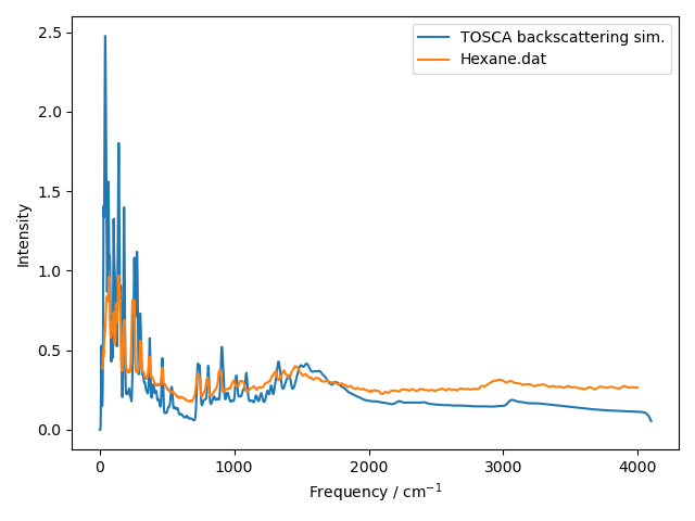
With a bit of arbitrary scaling in the ref_scale variable we get a nice comparison:

Note that the TXFA instrument pre-dates TOSCA; while the geometry is similar to the TOSCA backscattering bank, we expect the resolution to be broader and the background to be higher.

The agreement of many peaks is excellent for a general-purpose potential. Do have a try with some different models, not all of them will match experiment this way! One might also look at the effect of changing supercell dimensions and displacement sizes.

References

[1]

D. P. Kovács et al. (2023) “MACE-OFF23: Transferable Machine Learning Force Fields for Organic Molecules” https://arxiv.org/abs/2312.15211

[2]

I. Batatia et al. (2024) “A foundation model for atomistic materials chemistry” https://arxiv.org/abs/2401.00096

[3]

D. A. Braden et al. (1999) “Inelastic neutron scattering spectra of the longitudinal acoustic modes of the normal alkanes from pentane to pentacosane” J. Chem. Phys. 111, 429-437 https://doi.org/10.1063/1.479293